Materials+ML Workshop Day 7

Content for today:

• Supervised Learning Review

  • Regression, Logistic Regression, Classification
  • Train/validation/Test sets

• Regression Models

  • Linear Regression
  • High-dimensional Embeddings
  • Kernel Machines (if time)

• Application: Predicting Material Bandgaps

  • Applying Regression Models (if time)

Tentative Workshop Schedule:

Session	Date	Content
Day 0	06/16/2023 (2:30-3:30 PM)	Introduction, Setting up your Python Notebook
Day 1	06/19/2023 (2:30-3:30 PM)	Python Data Types
Day 2	06/20/2023 (2:30-3:30 PM)	Python Functions and Classes
Day 3	06/21/2023 (2:30-3:30 PM)	Scientific Computing with Numpy and Scipy
Day 4	06/22/2023 (2:30-3:30 PM)	Data Manipulation and Visualization
Day 5	06/23/2023 (2:30-3:30 PM)	Materials Science Packages
Day 6	06/26/2023 (2:30-3:30 PM)	Introduction to ML, Supervised Learning
Day 7	06/27/2023 (2:30-3:30 PM)	Regression Models
Day 8	06/28/2023 (2:30-3:30 PM)	Unsupervised Learning
Day 9	06/29/2023 (2:30-3:30 PM)	Neural Networks
Day 10	06/30/2023 (2:30-3:30 PM)	Advanced Applications in Materials Science

Questions

• Intro to ML Content:
  • Statistics Review
  • Linear Algebra Review
• Supervised Learning
  • Models and validity
  • Training, validation, and test sets
  • Normalizing Data
  • Gradient Descent
  • Classification Problems

Types of Machine Learning Problems

Machine Learning Problems can be divided into three general categories:

• Supervised Learning: A predictive model is provided with a labeled dataset with the goal of making predictions based on these labeled examples
  • Examples: regression, classification

• Unsupervised Learning: A model is applied to unlabeled data with the goal of discovering trends, patterns, extracting features, or finding relationships between data.
  • Examples: clustering, dimensionality reduction, anomaly detection

• Reinforcement Learning: An agent learns to interact with an environment in order to maximize its cumulative rewards.
  • Examples: intelligent control, game-playing, sequential design

Supervised Learning

• Learn a model that makes accurate predictions $\hat{y}$ of $y$ based on a vector of features $\mathbf{x}$.

• We can think of a model as a function $f : \mathcal{X} \rightarrow \mathcal{Y}$

  • $\mathcal{X}$ is the space of all possible feature vectors $\mathbf{x}$
  • $\mathcal{Y}$ is the space of all labels $y$.

Problems with Model Validity

• Even if a model fits the dataset perfectly, we may not know if the fit is valid, because we don't know the $(\mathbf{x},y)$ pairs that lie outside the training dataset:

Traning Validation, and Test Sets:

• Common practice is to set aside 10% of the data as the validation set.
• In some problems another 10% of the data is set aside as the test set.

Validation vs. Test Sets:

• The validation set is used for comparing the accuracy of different models or instances of the same model with different parameters.

• The test set is used to provide a final, unbiased estimate of the best model selected using the validation set.

Preparing Data:

• To avoid making our model more sensitive to features with high variance, we normalize each feature, so that it lies roughly on the interval $[-2,2]$.

• Normalization is a transformation $\mathbf{x} \mapsto \mathbf{z}$:

$$z_i = \frac{x_i - \mu_i}{\sigma_i}$$

• $\mu_i$ and $\sigma_i$ are the mean and standard deviation of the $i$th feature in the training dataset.

Model Loss Functions:

• We can evaluate how well a model $f$ fits a dataset $\{(\mathbf{x}_i, y_i)\}_{i=1}^N$ by taking the average of a loss function evaluated on all $(\mathbf{x}_i, y_i)$ pairs.

Examples:

• Mean Square Error (MSE):

  $$\mathcal{E}(f) = \frac{1}{N} \sum_{n=1}^N (f(\mathbf{x}_n) - y_n)^2$$

• Mean Absolute Error (MAE):

  $$\mathcal{E}(f) = \frac{1}{N} \sum_{n=1}^N |f(\mathbf{x}_n) - y_n|$$

• Classification Accuracy:

  $$\mathcal{E}(f) = \frac{1}{N} \sum_{n=1}^N \delta(\hat{y} - y) = \left[ \frac{\text{# Correct}}{\text{Total}} \right]$$

Gradient Descent

• Gradient descent makes iterative adjustments to the model weights $\mathbf{w}$:

$$\mathbf{w}^{(t+1)} = \mathbf{w}^{(t)} - \nabla_w \mathcal{E}(f)$$

Today's Content:

Advanced Regression Models

• Multivariate Linear Regression
  • High-Dimensional Embeddings
• Regularization
  • Undervitting vs. overfitting
  • Ridge regression
• Kernel Machines (if time)
  • Support Vectors
  • Kernel Functions
  • Support Vector Machines
• Application:
  • Predicting Bandgaps of Materials

Multivariate Linear Regression

• Multivariate Linear regression is a type of regression model that estimates a label as a linear combination of features:

$$\hat{y} = f(\mathbf{x}) = w_0 + \sum_{i=1}^D w_i x_i$$

• If $\mathbf{x}$ has $D$ features, there are $D+1$ weights we must determine to fit $f$ to data.

• We can re-write the linear regression model in vector form:

  • Let $\underline{\mathbf{x}} = \begin{bmatrix} 1 & x_1 & x_2 & \dots & x_D \end{bmatrix}^T$ ($\mathbf{x}$ padded with a 1)
  • Let $\mathbf{w} = \begin{bmatrix} w_0 & w_1 & w_2 & \dots & w_D \end{bmatrix}^T$ (the weight vector)

• $f(\mathbf{x})$ is just the inner product (i.e. dot product) of these two vectors:

$$\hat{y} = f(\mathbf{x}) = \underline{\mathbf{x}}^T\mathbf{w}$$

• For these linear regression models, it is helpful to represent a dataset $\{ (\mathbf{x}_n,y_n) \}_{n=1}^N$ as a matrix-vector pair $(\mathbf{X},\mathbf{y})$, given by:

$$\mathbf{X} = \begin{bmatrix} \underline{\mathbf{x}_1}^T \\ \underline{\mathbf{x}_2}^T \\ \vdots \\ \underline{\mathbf{x}_N}^T \end{bmatrix},\qquad\qquad \mathbf{y} = \begin{bmatrix} y_1 \\ y_2 \\ \vdots \\ y_N \end{bmatrix}$$

• This is helpful because it allows us to write the MSE (mean square error) model loss function in matrix form:

$$\text{MSE}: \mathcal{E}(f) = \frac{1}{N} \sum_{n=1}^N (\hat{y} - y)^2$$

• In terms of $\mathbf{X}$ and $\mathbf{y}$, we write:

$$\mathcal{E}(f) = \frac{1}{N}(\mathbf{X}\mathbf{w} -\mathbf{y})^T(\mathbf{X}\mathbf{w} - \mathbf{y})$$

• It can be shown that the weight vector $\mathbf{w}$ minimizing the MSE $\mathcal{E}(f)$ can be computed in closed form:

$$\mathbf{w} = \mathbf{X}^+\mathbf{y}$$

• Above, $\mathbf{X}^+$ denotes the Moore-Penrose inverse (sometimes called the pseudo-inverse) of $\mathbf{X}$.

• If the dataset size $N$ is sufficiently large such that $\mathbf{X}$ has linearly independent columns, the optimal weights can be computed as:

$$\mathbf{w} = \mathbf{X}^{+}\mathbf{y} = \left( (\mathbf{X}^T\mathbf{X})^{-1}\mathbf{X}^T\right)\mathbf{y}$$

High-Dimensional Embeddings

• Often, the trends of $y$ with respect to $\mathbf{x}$ are non-linear, so multivariate linear regression may fail to give good results.

• One way of handling this is by embedding the data in a higher-dimensional space using many different non-linear functions:

$$\phi_j(\mathbf{x}) : \mathbb{R}^{D} \rightarrow \mathbb{R}\qquad (j = 1, 2, ..., D_{emb})$$

(The $\phi_j$ are nonlinear functions, and $D_{emb}$ is the embedding dimension)

• After embedding the data in a $D_{emb}$-dimensional space, we can apply linear regression on to the embedded data:

$$\hat{y} = f(\mathbf{x}) = w_0 + \sum_{j=1}^{D_{emb}} w_j \phi_j(\mathbf{x})$$

• The loss function used in these models is also commonly the mean square error (MSE):

$$\mathcal{E}(f) = \frac{1}{N}(\mathbf{\Phi}(\mathbf{X})\mathbf{w} - \mathbf{y})^T(\mathbf{\Phi}(\mathbf{X})\mathbf{w} - \mathbf{y})$$

• Above, the quantity $\Phi(\mathbf{X})$ is the embedding of the data matrix $\mathbf{X}$. It is a matrix with the following form:

$$\mathbf{\Phi}(\mathbf{X}) = \begin{bmatrix} 1 & \phi_1(\mathbf{x}_1) & \phi_2(\mathbf{x}_1) & \dots & \phi_{D_{emb}}(\mathbf{x}_1) \\ 1 & \phi_1(\mathbf{x}_2) & \phi_2(\mathbf{x}_2) & \dots & \phi_{D_{emb}}(\mathbf{x}_2) \\ \vdots & \vdots & \vdots & \ddots & \vdots \\ 1 & \phi_1(\mathbf{x}_N) & \phi_2(\mathbf{x}_N) & \dots & \phi_{D_{emb}}(\mathbf{x}_N) \end{bmatrix}$$

• Fitting a linear regression model in a high-dimensional space can be computationally expensive:

$$\hat{y} = f(\mathbf{x}) = w_0 + \sum_{j=1}^{D_{emb}} w_j \phi_j(\mathbf{x})$$$$\mathbf{w} = \Phi(\mathbf{X})^+\mathbf{y}$$

• This is especially true if $D_{emb} \gg D$.

Example: Fitting polynomials:

• To fit a polynomial to 1D $(x_i, y_i)$ data, we can use the following embedding matrix:

$$\mathbf{\Phi}(\mathbf{X}) = \begin{bmatrix} 1 & x_1 & x_1^2 & \dots & x_1^{D_{emb}} \\ 1 & x_2 & x_2^2 & \dots & x_2^{D_{emb}} \\ 1 & x_3 & x_3^2 & \dots & x_3^{D_{emb}} \\ \vdots & \vdots & \vdots & \ddots & \vdots \\ 1 & x_N & x_N^2 & \dots & x_N^{D_{emb}} \end{bmatrix}$$

• This matrix is referred to as a Vandermonde matrix.

Underfitting and Overfitting

• High-dimensional embeddings are powerful because they give a model enough degrees of freedom to conform to non-linearities in the data.

• The more degrees of freedom a model has the more prone it is to "memorizing" the data instead of "learning from it".

• Fitting a model requires striking a balance between these two extremes.

• A model underfits the data if it has insufficient degrees of freedom to model the data.
  • Underfitting often results from poor model choice.
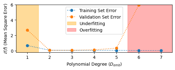
  • When underfitting occurs, both the training and validation error are very high

• A model overfits the data if it has too many degrees of freedom such that it fails to generalize well outside of the training data.
  • Overfitting results from applying a model that is too complex to a dataset that is too small.
  • When overfitting occurs, the training error plateaus at a minimum (typically at zero) and the validation error increases suddenly.

Example: Polynomial Regression

• We can diagnose underfitting and overfitting by evaluating the training and validation error as a function of model complexity (in this case, $D_{emb}$).

Polynomial Regression Example:

Regularization:

• One way of reducing overfitting is by gathering more data.

  • Having more data makes it harder for a model to "memorize" the entire dataset.

• Another way to reduce overfitting is to apply regularization

  • Regularization refers to the use of some mechanism that deliberately reduces the flexibility of a model in order to reduce the validation set error

  • A common form of regularization is penalizing the model for having large weights.

• For most models, a penalty term is added to the overall model loss function.

  • The model minimizes the loss while not incurring too large of a penalty:

  $$\text{ Penalty Term } = \lambda \sum_{j} w_j^2 = \lambda(\mathbf{w}^T\mathbf{w})$$

• The parameter $\lambda$ is called the regularization parameter

  • as $\lambda$ increases, more regularization is applied.

Ridge Regression

• Ridge Regression is a form of regression directly adds this regularization term to the MSE:

$$\mathcal{E}(f) = \frac{1}{N}(\mathbf{\Phi}(\mathbf{X})\mathbf{w} - \mathbf{y})^T(\mathbf{\Phi}(\mathbf{X})\mathbf{w} - \mathbf{y}) + \underbrace{\lambda(\mathbf{w}^T\mathbf{w})}_{\text{regularization term}}$$

• For any value of $\lambda$ the optimal weights $\mathbf{w}$ for a ridge regression problem can be computed in closed form:

$$\mathbf{w} = \left((\mathbf{\Phi}(\mathbf{X})^T\mathbf{\Phi}(\mathbf{X}) + \lambda\mathbf{I})^{-1} \mathbf{\Phi}(\mathbf{X})^T \right) \mathbf{y}$$

Kernel Machines

• Kernel machines are an equivalent form of high-dimensional embedding models that avoid computing an embedding entirely:

$$ f(\mathbf{x}) = w_0 + \sum_{i=1}^{D_{emb}} w_i\phi_i(\mathbf{x})\quad \Rightarrow \quad f(\mathbf{x}) = w_0 + \sum_{n=1}^N (\alpha_n - \alpha_n^*)K(\mathbf{x}_n,\mathbf{x})$$

• Instead of enbedding data directly, kernel machines compute only the inner products of pairs of data points in the embedding space.

• This inner product is computed by a _kernel function $K(\mathbf{x}, \mathbf{x}')$.

• Kernel machines even allow us to perform linear regression in infinite dimensional spaces!

Tutorial: Bandgap Prediction

• We will work with some data obtained from the Materials Project database to develop a model that predicts the bandgap of materials.

Recommended Reading:

• Unsupervised Learning

If possible, try to do the exercises. Bring your questions to our next meeting tomorrow.