Basic Neural Networks#
In this section we will describe in greater detail how a basic neural network model works and why a neural network has greater flexibility than some of the models we have studied previously. This flexibility, however, often comes at the cost of low interpretability, as generating a simple explanation of why a large neural network makes a particular prediction is often quite difficult.
In this section we will learn some basic principles about neural networks and then implement a densely-connected feed-forward neural network using the popular machine learning framework Pytorch.
A Single Neuron#
In previous sections, we encountered the linear classifier model (or Perceptron), which had the following form:
where \(\text{sign}(x) = \begin{cases} +1 & x > 0\\ -1 & x <= 0 \end{cases}\).
Originally, the perceptron model was inspired by the biological function of a multipolar neuron, which produces an electrical response (the “output” of the neuron) if a weighted sum of electrical stimuli from neighboring neurons (the “inputs” of the neuron) exceed a given threshold. In this model of a neuron, the function that dictates the neuron’s response with respect to the sum of inputs is referred to as a neuron activation function, which we will denote here as \(\sigma(x)\). This activation function is applied before the neuron outputs a response, as shown in the diagram below:

More generally, the output of a single neuron with weight vector \(\mathbf{w} = \begin{bmatrix} w_0 & w_1 & \dots & w_D \end{bmatrix}^T\) and activation function \(\sigma(x)\) can be written as follows:
(Recall that \(\underline{\mathbf{x}}\) is the vector \(\mathbf{x}\) prepended with \(1\): \(\underline{\mathbf{x}} = \begin{bmatrix} 1 & x_1 & x_2 & \dots & x_D \end{bmatrix}\))
Activation Functions:#
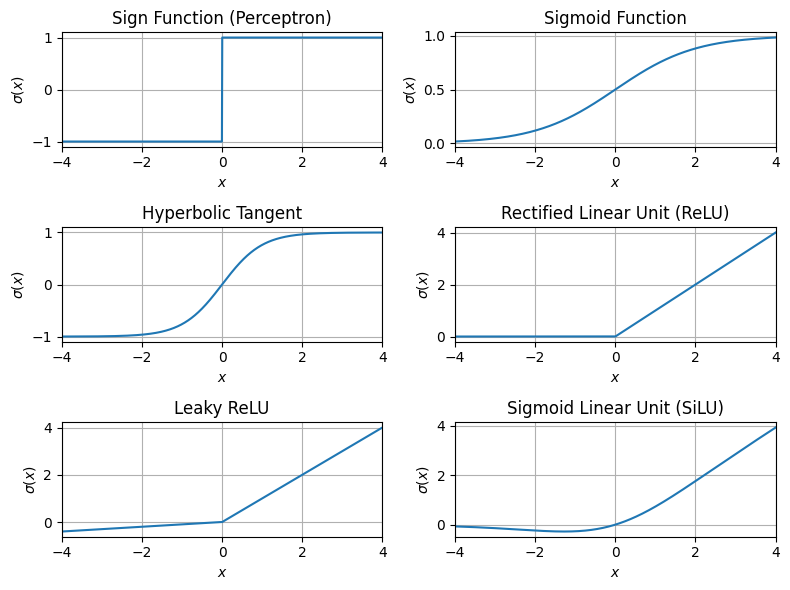
In order for a network of neurons to “learn” from non-linear data, it is critical that the neuron activation function \(\sigma(x)\) is non-linear. For example, in the perceptron model, the activation function is \(\sigma(x) = \text{sign}(x)\), which fits this criterion. However, this function is not continuous, and its derivative is \(0\) almost everywhere. In order to fit a neural network to data though a method such as gradient descent, it is desirable that the activation function \(\sigma(x)\) be both continuous and differentiable. Below, we give some alternative activation functions that are commonly used in neural networks:
Sigmoid function:
Hyperbolic Tangent:
Rectified Linear Unit (ReLU):
Leaky ReLU:
(\(\alpha\) is chosen such that \(0 < \alpha \ll 1\). Typically, \(\alpha = 10^{-3}\))
Sigmoid Linear Unit (SiLU) :
The activation function used is chosen depending on the kind of outputs desired for each neuron and the kind of model being used. In most cases, the ReLU activation function is a good choice.
Below, we write some Python code that visualizes each of these activation functions:
Show code cell source
import numpy as np
import matplotlib.pyplot as plt

# define activation functions:
activation_functions = {
    'Sign Function (Perceptron)': lambda x : np.sign(x),
    'Sigmoid Function': lambda x : 1/(1 + np.exp(-x)),
    'Hyperbolic Tangent': lambda x : np.tanh(x),
    'Rectified Linear Unit (ReLU)': lambda x : np.maximum(0,x),
    'Leaky ReLU': lambda x : np.maximum(0.1*x, x),
    'Sigmoid Linear Unit (SiLU)': lambda x : x / (1 + np.exp(-x))
}

# plot each activation function:
plt.figure(figsize=(8,6))
for i, (name,sigma) in enumerate(activation_functions.items()):
    plt.subplot(3,2,i+1)
    x = np.linspace(-4, 4, 1000)
    y = sigma(x)
    plt.grid()
    plt.xlim(-4,4)
    plt.plot(x,y)
    plt.title(name)
    plt.xlabel(r'$x$')
    plt.ylabel(r'$\sigma(x)$')

plt.tight_layout()
plt.show()
Note
When choosing an activation function for the last layer of a neural network, be sure that the range of the final activation function matches the range of data. For example, if your model is predicting probabilities (or probability distributions), then a sigmoid activation function may be the most appropriate.
If a neural network model is performing regression and there is no bound on the range of predicted values, then an activation function is not applied to the last layer.
Networks of Neurons#
By networks of individual neurons into layers and stacking these layers, we can produce some very powerful non-linear models. Layered neural network models can be applied to almost any supervised learning task, even tasks where the there are multiple labels that need to be predicted (i.e. where \(\mathbf{y}\) is a vector, not just a scalar).
The simplest kind of neural network layer we can construct is a fully-connected layer, in which a collection of neurons produce a vector of outputs \(\mathbf{a}\) (where each element \(a_i\) corresponds to a single neuron output) based on different linear combinations of the input features. Specifically, a layer of \(m\) neurons can be used to compute the function:
Above \(w_{i,j}\) (sometimes written \(w_{ij}\)) denotes weight of feature \(j\) in neuron \(i\). In total, this layer of neurons has \(m \times (D+1)\) weights, which we can organize into a rectangular weight matrix \(\mathbf{W}\) as follows:
In terms of this weight matrix, we can write the layer’s function as a matrix-vector product, namely:
(Note that when we write \(\sigma(\mathbf{A})\) where \(\mathbf{A}\) is a matrix or vector, it denotes that the activation function \(\sigma\) is applied element-wise; that is, to each entry of \(\mathbf{A}\) individually.)
A standard feed-forward neural network is a simple kind of neural network that stacks two layers of neurons; the first layer computes a vector of features \(\mathbf{a}\) from the data \(\mathbf{x}\). This layer is sometimes called a hidden layer. Next, a second layer computes the output vector \(\hat{\mathbf{y}}\). (In the case where only a single output is desired, only one neuron is used in the output layer to output a scalar value \(\hat{y}\).) Here, we will let \(\mathbf{W}\) denote the weight matrix of the hidden layer, and \(\mathbf{V}\) denote the weight matrix of the second layer. We can visualize this network and the connectedness between neuron layers as follows:

By composing the equations for the hidden layer inside the equation for the output layer, we obtain the final model equation for a standard feed-forward neural network: