Supervised Learning#
Now that we have reviewed some of the necessary background material, we will begin examining the most common type of machine learning problem: supervised learning. Supervised learning is applied to problems where the available data contains many different labeled examples, and the problem involves finding a model that maps a set of features (inputs) to labels (outputs).
Although data can take many different forms (i.e. numbers, vectors, images, text, 3D structures, etc.), we can think of a dataset as a collection of \((\mathbf{x}, y)\) pairs, where \(\mathbf{x}\) is a set of features, and \(y\) is the label to be predicted. For now, we will consider the simplest case where \(\mathbf{x}\) is a vector of floating-point numbers and \(y\) is either (a) one of a finite number of mutually exclusive classes, or (b) a scalar quantity. In case (a), the supervised learning problem is a classification problem, where we must learn a model that makes prediction \(\hat{y}\) of the class \(y\) associated with the set of features \(\mathbf{x}\). In case (b), the supervised learning problem is a regression problem, where we must learn a model that produces an estimate \(\hat{y}\) of \(y\) based on \(\mathbf{x}\).
For both classification and regression problems, we can think of a model as a function \(f: \mathcal{X} \rightarrow \mathcal{Y}\) that maps the space of possible features \(\mathcal{X}\) into the space of possible labels \(\mathcal{Y}\).

Ideally, we would like the function \(f\) to be a valid model. We define a model to be valid if it correctly predicts labels across the entire domain \(\mathcal{X}\). In practice, this means generalizing well to both seen and unseen data; however, finding such a function may be difficult for a number of reasons. First, it is possible that \(\mathcal{X}\) might be an infinite set, meaning it is impossible to verify that \(f\) is valid for all sets of features \(\mathbf{x}\). In some situations, we may not even know what the correct labels are for every single \(\mathbf{x}\). For these reasons, it might appear that learning a valid model \(f: \mathcal{X} \rightarrow \mathcal{Y}\) is an impossible challenge.
Fortunately, we have a powerful tool that we can use to tackle this seemingly insurmountable task: data. Using the data we have gathered, we can estimate the validity of a model by determining how well it fits the data. Quantitatively speaking, we say that a model \(f\) fits a dataset of \((\mathbf{x}_i,y_i)\) pairs if \(f(\mathbf{x}_i) \approx y_i\) for each \(i\).
We also know that following statement is generally true with regards to our data and any potential model \(f\):
If a model \(f : \mathcal{X} \rightarrow \mathcal{Y}\) is valid, then it will fit the data.
Indeed, any model that is valid should produce a good fit to the data, provided that enough features are accounted for in \(\mathcal{X}\) and that sufficient care is taken to eliminate noise in the data.
Now, take a moment to consider the converse of the previous statement:
If a model \(f : \mathcal{X} \rightarrow \mathcal{Y}\) fits the data, then it is valid.
The converse statement is not generally true. In fact, sometimes a model that fits the data better than another model may actually be less valid. For example, a model could be matching noise in the data without capturing the underlying pattern. To illustrate this point, consider the following regression problem, where we have proposed two different fits:
Show code cell source
import numpy as np
import matplotlib.pyplot as plt

# seed random number generator
np.random.seed(0)

# define data distribution:
def y_distribution(x):
	return -0.1*x + 0.9 + \
            np.random.uniform(-0.3,0.3,size=len(x))

# the data we obtain will naturally fit the valid model with
# some noise due to experimental errors:
data_n = 12
data_x = np.linspace(0,10,data_n)
data_y = y_distribution(data_x)

# fit data to a line (degree 1 polynomial):
xy_linefit = np.poly1d(np.polyfit(data_x,data_y,deg=1))

# fit data to N-1 degree polynomial to data:
xy_polyfit = np.poly1d(np.polyfit(data_x,data_y,deg=len(data_x)-1))

# plot data and valid/invalid models for comparison:
plt.figure()
eval_x = np.linspace(0,10,1000)
plt.scatter(data_x,data_y, color='g', label=r'Data $(x,y)$')
plt.plot(eval_x, xy_linefit(eval_x), label=r'Linear Fit $f(x)$')
plt.plot(eval_x, xy_polyfit(eval_x), label=r'Polynomial Fit $f(x)$')
plt.xlabel('x')
plt.ylabel('y')
plt.legend()
plt.show()
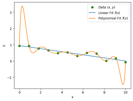
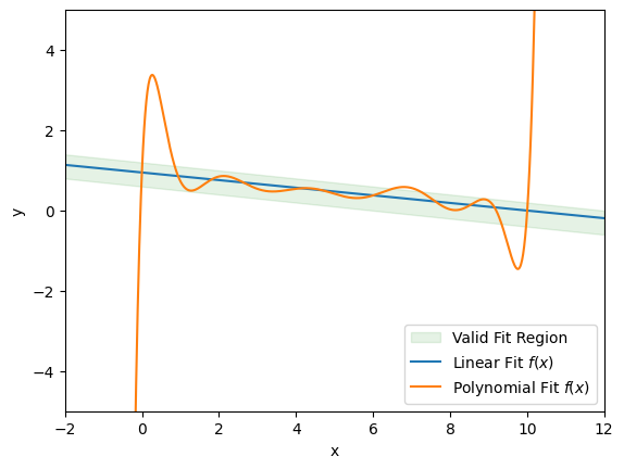
Above, we have randomly generated data and proposed two models: a linear fit of the form \(f(x) = mx + b\) and a degree 11 polynomial fit of the form \(f(x) = \sum_{n=0}^{11} a_n x^n\). Since a polynomial of degree \(N-1\) can perfectly fit \(N\) data points, the fit exactly matches the data, whereas the linear fit does not. Nonetheless, it is likely that a linear fit is the more valid model, especially when we consider that the polynomial fit extrapolates very poorly outside of the interval \([0,10]\) that contained the dataset.
Show code cell source
# determine the region of valid fits:
extrap_x = np.linspace(-2, 12, 1000)
valid_fit_region = [
    -0.1*extrap_x + 0.9 - 0.3,
    -0.1*extrap_x + 0.9 + 0.3
]

# plot how well the fits extrapolate from the data:
plt.figure()
plt.fill_between(extrap_x, valid_fit_region[0], valid_fit_region[1],
                 color='g', alpha=0.1, label='Valid Fit Region')
plt.plot(extrap_x, xy_linefit(extrap_x), label=r'Linear Fit $f(x)$')
plt.plot(extrap_x, xy_polyfit(extrap_x), label=r'Polynomial Fit $f(x)$')
plt.xlim((-2,12))
plt.ylim((-5,5))
plt.xlabel('x')
plt.ylabel('y')
plt.legend()
plt.show()
From this exercise, we see that some models are not valid, even though they may perfectly fit the data. So if we have a model that does seem to fit the data set well, how can we be sure that the model is also valid? Unfortunately, we can never know the degree to which a model is valid unless our dataset contains every possible input in \(\mathcal{X}\) and its associated label. However, there are some general tactics we can employ to maximize the validity of our model. These are the three most important guidelines to keep in mind when working with supervised models:
Be mindful of how the data is obtained.
Is the data accurate? Are sources of noise identified and accounted for? Does the dataset adequately span the set of relevant input features \(\mathcal{X}\) and labels \(\mathcal{Y}\)? You can never have too much data, but you can have too much redundant or unbalanced data.
Be mindful of how the data is handled.
How is the data handled to fit the model? Are training, validation, and test sets being used, and are they kept independent of one another? Are you avoiding selection bias? If you are enriching the dataset with additional features, are those features necessary and accurate?
Be sure that an appropriate model is being used.
Does the size of the dataset warrant the complexity of the model you are using? Are any symmetries of the data reflected in the symmetries of the model?
Obtaining Data#
Depending on the problem you are investigating, you may or may not play a role in the data collection process. Since we are materials scientists, the data we are working with often comes from either laboratory measurements or computational simulations. If you happen to have some control over the data collection process, make every effort to ensure that the data is collected in a consistent manner, and that meaningful features and labels are reported accurately for each laboratory sample. If you are generating data through computational simulations, be sure that any data produced is at least consistent with values measured in the laboratory or with other independently reported values in the literature. After all, your aim is to develop a model of the physics and chemistry of the real world, not a model of the (often simplified) physics and chemistry of a simulation. As a famous computational scientist once said:
“The purpose of computing is insight, not numbers.”
—Richard Hamming
If you are collecting data for a classification problem, make sure that all classes are represented in a balanced ratio, if possible. This will help a model avoid bias toward predicting the classes that appear more frequently in the dataset. Likewise, for regression problems be sure that the extremes of both \(\mathcal{X}\) and \(\mathcal{Y}\) are contained in the dataset. This will help mitigate extrapolation error, as we saw in the previous example with the polynomial fit.
Handling Data#
Let’s return to the problem of determining model validity. We said earlier that a model \(f\) is valid if \(f(\mathbf{x}) = \hat{y} \approx y\) for points \(\mathbf{x}\) both inside and outside of the dataset. However, we do not know what the correct values in \(\mathcal{Y}\) that correspond to feature sets \(\mathbf{x}'\) lying outside the dataset:

Without data that is kept separate from the data that the model was fit to, we have no way of estimating the validity of the model, that is, how accurate the model is on \(\mathcal{X}\) as a whole, not just on the dataset used to fit the model. This is why it is customary to set aside a subset of the data that is not used for fitting the model, but is used for only ensuring the validity of the model. This reserved subset of the dataset is usually referred to as the validation set. By measuring the model’s accuracy on the validation set, we can effectively estimate how well the model generalizes to data that was not used. When using the validation set, we must be careful, since this estimate is only valid if the dataset provides sufficient coverage of the set of possible input features \(\mathcal{X}\). In other words, any biases present in the dataset will result in biases in the estimates of model accuracy obtained by a validation set.
Today, it has become best practice in most supervised machine learning problems to split the dataset into three randomly selected independent subsets: a training set, a validation set, and a test set. Typically, these subsets comprise 80%, 10%, and 10% of the total dataset respectively:

Let’s take a look at each of these three subsets and their importance in supervised learning:
The Training Set#
The training set comprises most of our dataset, and rightfully so. It contains the data that we fit our model to (often the process of fitting a model to data is referred to as training). Later in this workshop we will discuss some of the algorithms used to train various models.
As a general rule of thumb for large datasets, the training set should be about 80% of the data. For some smaller datasets you may want to instead use only 60-70% to ensure the validation and test sets are large enough.
The Validation Set#
The validation set is used to evaluate the accuracy of multiple configurations of the same model and to select the best one. Models can have many parameters that affect how flexible or inflexible the model is. For example, the degree of a polynomial fitted to one-dimensional data can be increased to make the model more flexible, but this flexibility can reduce the model’s ability to make predictions outside of the training set. To find the optimal configuration of these parameters, multiple models are trained on the training set and their accuracies on the validation set are compared. As its name suggests, the validation set plays an important role in ensuring that the model is valid and can make predictions that generalize well outside the training set.
The Test Set#
Since the validation set is used to evaluate and select the best of many different models with different parameters, it is possible that the process of selecting the best model can introduce selection bias into the estimate that the validation set provides of the overall model’s performance. Selection bias can become increasingly problematic as the number of models evaluated on the same validation set increases. This is why we set aside a third subset of the data: the test set. The test set is used to provide a final unbiased evaluation of the model. It should never be used as a basis for comparing multiple models.
Standardizing Data#
When working with datasets containing many different features, the differences in the numerical scale of each feature can cause the model to be more sensitive to some features and less sensitive to others. Sometimes, even changing the units of the features can significantly affect the accuracy of a model. To avoid this problem and ensure that the accuracy of the model is invariant under how the data is scaled, we use a technique called data standardization.
Data standardization works as follows: instead of fitting a model to a training set consisting of \((\mathbf{x}, y)\) pairs, we fit the model to a transformed dataset, consisting of pairs \((\mathbf{z}, y)\), where the \(i\)th entry of \(\mathbf{z}\) is given by:
Above, \(\mu_i, \sigma_i\) are the mean and standard deviation of the \(i\)th component of the training set features. After standardization, all features will have values roughly on the interval \([-2, 2]\). This ensures that each feature makes an equally-weighted contribution to any predictions made.
Model Selection#
The task of finding the best model for a supervised learning problem is generally quite difficult. Unfortunately, there is no tried and true method for determining which model is most appropriate for a specific supervised learning problem. Finding the best model often requires a combination of trial-and-error and expertise in both the dataset and the problem being studied. The good news is that as materials scientists, the kinds of supervised learning problems we encounter in our research often have some underlying physical theory that we can apply directly to the data. Sometimes, by adding some free parameters to these physically informed models, we can obtain a good fit of the data that generalizes well outside the training set. It may also be the case that similar supervised learning problems have been studied before, and a paper or two has been published, along with details of the models used. When it comes to selecting a few models worth trying, a good guiding principle is Occam’s Razor:
“Entities must not be multiplied beyond necessity.”
—Occam’s Razor
In the context of machine learning, Occam’s razor is often interpreted as follows: Models with few free parameters and low complexity should be preferred over complex models, unless simple models fail to give good results. When trying to find the best model, start with simple models, and gradually increase the complexity. For each model you want to evaluate, fit it to the training set data and evaluate its accuracy on the validation set. If your model performs poorly, try some more complex models and see if the validation set accuracy increases. As you obtain more experience working with the kinds of models most often used in your field, you will gain more intuition about which models work better than others.
Exercises#
Exercise 1: Training, Validation, and Test Sets
Let’s get some practice with preparing data. To keep things simple, use the dataset generated by the following code:
x_data = np.random.uniform(-30, 30, size=100)
y_data = 10 - 0.01*x_data**2 + np.random.normal(0,2,size=100)
To prepare this dataset for use with a model, do the following:
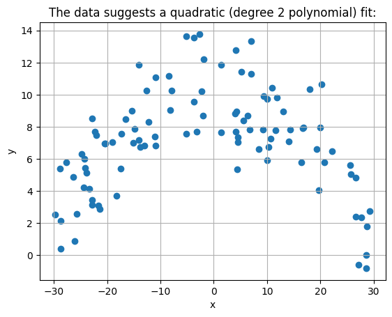
Plot the data. What kind of model might produce a good fit?
Split the dataset into training, validation and test sets with the standard 80%-10%-10% split. There are a few ways to do this. One way is by shuffling the data using Python’s
random.shuffleand selecting subsets of the data by their indices. Another (easier) way is to usesklearn.model_selection.train_test_split. This function can only split the data into two subsets, so you will need to use it twice: once to split off the training set and once more to split the remaining data into the validation and test sets.Standardize the training, validation, and test sets (transform \(x \rightarrow z\)). You can do this by computing \(\mu_x\) and \(\sigma_x\) with
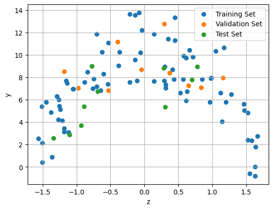
np.meanandnp.stdrespectively, or by usingsklearn.preprocessing.StandardScaler.Plot the standardized training, validation, and test sets on the same axes. Use a different color for each set.
Exercise 2: Polynomial Models
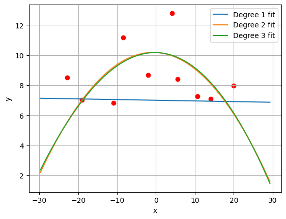
Using the standardized training, validation, and test sets from Exercise 1, generate three different fits using polynomials of degree 1, 2, and 3.
Visually inspect the fit of these three models by plotting the validation set and each fit on the same axes. (Plot the non-standardized \((x,y)\) data, not the standardized \((z,y)\) data.)
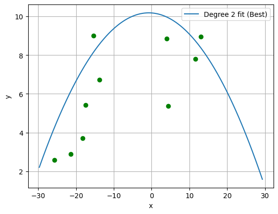
Finally, select the best fit and plot it on the same axes as the test set. When plotting your fit curves, be sure to standardize the inputs to your model before. (In the next section, we will discuss functions that can be used to quantitatively measure goodness of fit. For now, we will measure goodness of fit qualitatively with our eyeballs.)
Hint: As shown in the example code above, you can fit a polynomial of degree n to standardized data using np.polyfit:
# fit polynomial model to standardized data:
poly_model = np.poly1d(np.polyfit(z_data, y_data, deg=n))

# evaluate polynomial model at (standardized) point z:
yhat = poly_model(z)
Solutions:#
Exercise 1: Training, Validation, and Test Sets#
Show code cell content
import numpy as np
import matplotlib.pyplot as plt
from sklearn.model_selection import train_test_split

# This is the dataset we are given:
x_data = np.random.uniform(-30, 30, size=100)
y_data = 10 - 0.01*x_data**2 + np.random.normal(0,2,size=100)

# (1) plot dataset:
plt.figure()
plt.grid()
plt.scatter(x_data, y_data)
plt.xlabel('x')
plt.ylabel('y')
plt.title('The data suggests a quadratic (degree 2 polynomial) fit:')
plt.show()

# (2) Split dataset into training, validation, and test sets.
# First, split data into training and non-training data:
x_train, x_nontrain, y_train, y_nontrain = train_test_split(x_data, y_data, train_size=0.8)

# Further split non-training data into validation and test data:
x_validation, x_test, y_validation, y_test = train_test_split(x_nontrain, y_nontrain, test_size=0.5)

# (3) standardize the train/validation/test sets.
# Estimate mu and sigma for training set:
mu_x = np.mean(x_train)
sigma_x = np.std(x_train)

# standardize data:
z_train = (x_train - mu_x)/sigma_x
z_validation = (x_validation - mu_x)/sigma_x
z_test = (x_test - mu_x)/sigma_x

# standardize y data:
mu_y = np.mean(y_train)
sigma_y = np.mean(y_train)

# (4) Plot the standardized train/validation/test sets:
plt.figure()
plt.grid()
plt.scatter(z_train, y_train, label='Training Set')
plt.scatter(z_validation, y_validation, label='Validation Set')
plt.scatter(z_test, y_test, label='Test Set')
plt.xlabel('z')
plt.ylabel('y')
plt.legend()
plt.show()
Exercise 2: Polynomial Models#
Show code cell content
# fit polynomials of degrees 1,2, and 3 to standardized data:
poly_1 = np.poly1d(np.polyfit(z_train, y_train, deg=1))
poly_2 = np.poly1d(np.polyfit(z_train, y_train, deg=2))
poly_3 = np.poly1d(np.polyfit(z_train, y_train, deg=3))

# generate standardized points for evaluating the model:
x_eval = np.linspace(np.min(x_data), np.max(x_data), 1000)
z_eval = (x_eval - mu_x)/sigma_x

# evaluate models:
yhat_poly_1 = poly_1(z_eval)
yhat_poly_2 = poly_2(z_eval)
yhat_poly_3 = poly_3(z_eval)

# plot polynomial fits and validation set:
plt.figure()
plt.grid()
plt.scatter(x_validation, y_validation, color='r')
plt.plot(x_eval, yhat_poly_1, label='Degree 1 fit')
plt.plot(x_eval, yhat_poly_2, label='Degree 2 fit')
plt.plot(x_eval, yhat_poly_3, label='Degree 3 fit')
plt.xlabel('x')
plt.ylabel('y')
plt.legend()
plt.show()

# Note: The second degree and third degree polynomials fit the data
#       quite well and do not appear to differ much in accuracy. Per
#       Occam's razor, the second degree polynomial is the better
#       model because it has fewer parameters.

# plot best polynomial fit and test set:
plt.figure()
plt.grid()
plt.scatter(x_test, y_test, color='g')
plt.plot(x_eval, yhat_poly_2, label='Degree 2 fit (Best)')
plt.xlabel('x')
plt.ylabel('y')
plt.legend()
plt.show()