Feature Selection and Dimensionality Reduction#
Sometimes when we are working with large datasets with many features, it can be difficult to figure out which features are important and which are not. This is especially true in unsupervised learning problems where we have a dataset \(\mathbf{x}\), but no regression or classification target value \(y\). Fortunately, there are some powerful dimensionality analysis and reduction techniques that can be applied for these problems. Here, we will focus on the most popular of these techniques, principal component analysis (PCA).
The Correlation Matrix#
In order to identify and extract meaningful features from data, we must first understand how the data is distributed. If the data is standardized (i.e. the transformation \(\mathbf{x} \rightarrow \mathbf{z}\) is applied), then every feature has mean \(\mu = 0\) and standard deviation \(\sigma = 1\); however, significant correlations may still exist between features, making the inclusion of some features redundant. We can see the degree to which any pair of standardized features are correlated by examining the entries of the correlation matrix \(\bar{\Sigma}\), given by:
where \(\mathbf{z}_1, \mathbf{z}_2, .., \mathbf{z}_N\) is the standardized dataset.
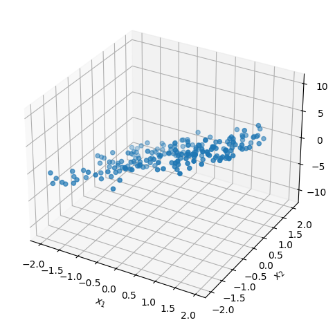
As a motivating example, let’s examine the correlation matrix of random 3D points that are approximately confined to the plane defined by the equation \(x_3 = 3x_1 -2x_2\). We can generate this dataset using the following Python code:
Important
The covariance matrix \(\Sigma\) is different from the correlation matrix \(\bar{\Sigma}\), though the two are commonly confused with one another. Both matrices are symmetric with entries given by:
The difference between these two matrices is the division by \(\sigma_i\sigma_j\) for \((i,j)\) entries.
Show code cell source
import numpy as np
import matplotlib.pyplot as plt

# set x3 as a linear combination of x1 and x2:
data_x1x2 = np.random.uniform(-2,2,size=(2,200))
data_x3 = np.dot(np.array([3,-2]),data_x1x2).reshape(1,-1)

# Add a little bit of noise to x3:
data_x3 += np.random.normal(0, 1, size=data_x3.shape)

# combine x1,x2,x3 features into a dataset (shape: (N,3)):
planar_data = np.vstack([ data_x1x2, data_x3 ]).T

# plot dataset in 3D:
plt.figure()
ax = plt.axes(projection='3d')
ax.scatter3D(planar_data[:,0],
             planar_data[:,1],
             planar_data[:,2])
ax.set_xlabel(r'$x_1$')
ax.set_ylabel(r'$x_2$')
ax.set_zlabel(r'$x_3$')
plt.tight_layout()
plt.show()
Next, we standardize the dataset and compute \(\bar{\Sigma}\) using np.cov:
Show code cell source
from sklearn.preprocessing import StandardScaler

# standardize data:
scaler = StandardScaler()
standardized_data = scaler.fit_transform(planar_data)

# compute the covariance matrix of the standardized data,
# which is called the correlation matrix:
cor_mat = np.cov(standardized_data.T)

# visualize covariance matrix:
max_cor = np.max(np.abs(cor_mat))
plt.matshow(cor_mat, cmap='seismic',
            vmin=-max_cor, vmax=max_cor)
for i, row in enumerate(cor_mat):
    for j, cor in enumerate(row):
        plt.text(i,j,f'{cor:.2f}', ha='center', fontsize=18)
features = [ r'$x_1$', r'$x_2$', r'$x_3$']
plt.gca().set_xticks([0,1,2])
plt.gca().set_yticks([0,1,2])
plt.gca().set_xticklabels(features)
plt.gca().set_yticklabels(features)
plt.show()
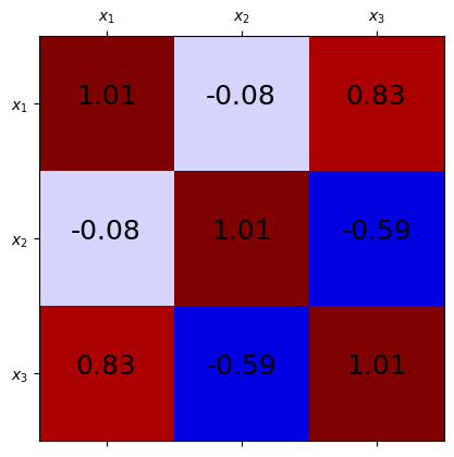
Examining the correlation matrix, we see strong positive correlation between \(x_1\) and \(x_3\) and strong negative correlation between \(x_2\) and \(x_3\), which corresponds to the relationship \(x_3 \approx 3x_1 - 2 x_2\). Since the third row of \(\bar{\Sigma}\) is highly correlated with the other features, it contributes the least to the overall variance of the data.
The Correlation Matrix in Supervised Learning
In supervised learning (where the dataset contains \((\mathbf{x},y)\) pairs, not just \(\mathbf{x}\) values) the correlation matrix and also be used to quantify the linear relationship between features and the output label \(y\). This is done by simply appending the corresponding \(y\) to the end of each \(\mathbf{x}\), standardizing this vector, and then computing the correlation matrix.
The values in this matrix that correspond to the correlation of \(y\) with each feature in \(\mathbf{x}\) can be used to reduce the dimensionality of the \(\mathbf{x}\) data. Specifically, features with the weakest correlation with \(y\) can be dropped, resulting in a much smaller feature vector. Since the dropped features had low correlation with \(y\), it is likely that it will not cause a drop in model accuracy. In fact, this will sometimes result an increase in model accuracy.
Principal Components Analysis#
Because the correlation matrix is symmetric, we can diagonalize the matrix by writing it as the product:
where \(\mathbf{D}\) is a diagonal matrix containing the eigenvalues of \(\bar{\Sigma}\) and \(\mathbf{P}\) is an orthogonal matrix (i.e. \(\mathbf{P}^T = \mathbf{P}^{-1}\)). The columns \(\mathbf{p}_1, \mathbf{p}_2, ..., \mathbf{p}_D\) of \(\mathbf{P}\) are called the principal components of the dataset. The principal components are vectors of magnitude \(1\) that are pairwise orthogonal, that is:
For our example dataset, we can compute the principal component matrix \(\mathbf{P}\) and eigenvalue matrix \(\mathbf{D}\) by diagonalizing \(\bar{\Sigma}\) as follows:
Show code cell source
# diagonalize the correlation matrix:
D_diag, P = np.linalg.eigh(cor_mat)

# make D_diag into a diagonal matrix:
D = np.diag(D_diag)

print('P matrix:')
print(P)

print('\nD matrix:')
print(D)

print('\nP @ D @ P.T (correlation matrix):')
print(P @ D @ P.T)
P matrix:
[[ 0.57733176  0.5773835  -0.57733555]
 [-0.38482472  0.81603255  0.43127812]
 [-0.72013747  0.02681757 -0.69331295]]

D matrix:
[[0.0286209  0.         0.        ]
 [0.         0.92789327 0.        ]
 [0.         0.         2.05856121]]

P @ D @ P.T (correlation matrix):
[[ 1.00502513 -0.08173477  0.82645711]
 [-0.08173477  1.00502513 -0.5872942 ]
 [ 0.82645711 -0.5872942   1.00502513]]
Each principal component \(\mathbf{p}_i\) (the \(i\)th column of \(\mathbf{P}\)) has an associated eigenvalue \(\lambda_i\), which is the corresponding value along the diagonal in the \(i\)th column of \(\mathbf{D}\). The eigenvalues \(\lambda_i\) describe the total variance of the data in the direction \(\mathbf{p}_i\). The principal component with the highest value of \(\lambda_i\) is called the first principal component, since it is a vector that points in the direction that “accounts for” most of the variance of the data. Similarly, the second principal component points in the direction that “accounts for” most of the variance not captured by the first principal component, and so on. Here, we will denote the first principal component as \(\mathbf{p}^{(1)}\), the second as \(\mathbf{p}^{(2)}\), and so on. We will use the same notation for the principal component eigenvalues, i.e. \(\lambda^{(1)}, \lambda^{(2)}\), etc.
From examining the printout of the \(\mathbf{D}\) matrix above, we see that \(\mathbf{p}^{(1)} = \mathbf{p}_3\) (the first principal component is the third column of \(\mathbf{P}\)) and \(\mathbf{p}^{(2)} = \mathbf{p}_2\) (the second principal component is the second column of \(\mathbf{P}\)). The corresponding eigenvalues are \(\lambda^{(1)} = 2.033\) and \(\lambda^{(2)} = 0.97\). However, we observe that \(\lambda^{(3)} = 0.024 \ll \lambda^{(1)}, \lambda^{(2)}\), which suggests that the third principal component accounts for very little variance in the data. This is due to the fact that the data is approximately confined to a 2D plane embedded in a larger 3D space.
One of the most powerful aspects of principal components analysis (often abbreviated PCA), is that we can project the standardized data onto the subset of principal components that are significant (i.e. have large \(\lambda_i\)), thereby reducing the dimensionality of the data while maximizing the amount of variance that is accounted for in the reduced data.
To project a standardized feature vector \(\mathbf{z}\) onto the first \(k\) principal components, we write it as a linear combination of all the principal components \(\mathbf{p}^{(1)}, ..., \mathbf{p}^{(D)}\):
Next, we solve for the coefficients \(u_i\). Since the \(\mathbf{p}^{(i)}\) are all orthonormal basis vectors, the coefficients can be computed independently of one another as follows:
The vector of the first \(k\) coefficients \(\mathbf{u} = \begin{bmatrix} u_1 & u_2 & ... & u_k \end{bmatrix}^T\) is the reduced \(k\)-dimensional representation of \(\mathbf{z}\). This vector is the projection of the data onto the first \(k\) principal components.
PCA Dimension Reduction#
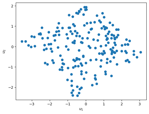
The sklearn Python package has functionality that makes PCA dimensionality reduction very easy. To compute the 2D PCA embedding of the 3D dataset we have been working on so far, we can use sklearn.decomposition.PCA, and visualize the projected data as follows:
Show code cell source
from sklearn.decomposition import PCA

# project standardized data onto the
# first two principal components:
pca = PCA(n_components=2)
pca.fit(standardized_data)
pc_data = pca.transform(standardized_data)

# plot projected data:
plt.figure()
plt.scatter(pc_data[:,0], pc_data[:,1])
plt.xlabel(r'$u_1$')
plt.ylabel(r'$u_2$')
plt.show()
Exercises#
Exercise 1: Applying PCA
Let’s get some practice working with PCA in the sklearn package. Consider the following 30-dimensional dataset sampled from a multivariate normal distribution:
from scipy.stats import ortho_group, multivariate_normal

# generate multivariate normal random dataset:
D = np.diag([1e-2]*20+list(np.random.uniform(1,10,10)))
U = ortho_group.rvs(D.shape[0])
mu = np.random.uniform(0,100, size=30)

data_x = multivariate_normal.rvs(mean=mu,cov=(U @ D @ U.T), size=4000)
To start, let’s try to determine the approximate dimensionality of the data. First, let’s take a look at all 30 principal components. Standardize the data and fit an instance of sklearn.decomposition.pca to it with n_components=30. Then take a look at the fitted PCA object’s explained_variance_ variable.
# fit a full PCA to data to determine explained variances:
full_pca = PCA(n_components=30)
full_pca.fit(data_z)

# extract explained variances (entries of D):
variances = full_pca.explained_variance_
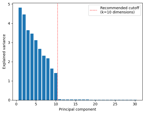
This is an array containing the eigenvalues of \(\bar{\Sigma}\) corresponding to each principal component (i.e. the diagonal of \(\mathbf{D}\) in sorted in descending order). Plot these values and try to determine the underlying dimensionality of the data (you should see a significant drop in explained variance at the number of underlying dimensions).
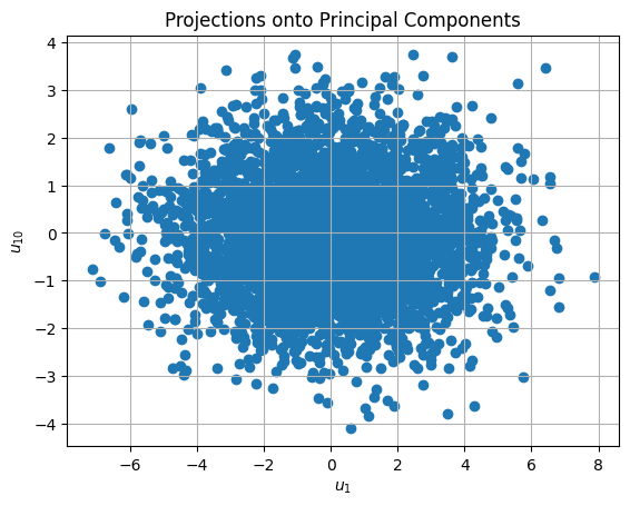
Once you determine the underlying number of dimensions, use a another PCA object with that number of components to reduce the dimensionality of the data. Plot the projections of the standardized data onto first and last of these principal components (i.e. \(u_1\) vs. \(u_k\), where \(k\) is the estimated dimensionality of the data).
Solutions#
Exercise 1: Applying PCA#
Show code cell content
from sklearn.decomposition import PCA
from sklearn.preprocessing import StandardScaler
from scipy.stats import ortho_group, multivariate_normal

# generate multivariate normal random dataset:
D = np.diag([1e-2]*20+list(np.linspace(1,3,10)**1.2))
U = ortho_group.rvs(D.shape[0])
mu = np.random.uniform(0,100, size=30)
data_x = multivariate_normal.rvs(mean=mu,cov=(U @ D @ U.T), size=4000)

# standardize dataset:
scaler = StandardScaler()
scaler.fit(data_x)
data_z = scaler.transform(data_x)

# fit a full PCA to data to determine explained variances:
full_pca = PCA(n_components=30)
full_pca.fit(data_z)

# extract explained variances (entries of D):
variances = full_pca.explained_variance_

# plot explained variance versus p.c. number:
plt.figure()
plt.bar(np.arange(1,len(variances)+1), variances)
plt.xlabel('Principal component')
plt.ylabel('Explained variance')
plt.axvline(10.5, color='r', linestyle=':', label='Recommended cutoff\n(k=10 dimensions)')
plt.legend()
plt.show()

# use a 10-dimensional PCA to reduce data:
partial_pca = PCA(n_components=10)
partial_pca.fit(data_z)
data_u = partial_pca.transform(data_z)

# plot u1 versus u10 to observe differences:
plt.figure()
plt.title('Projections onto Principal Components')
plt.grid()
plt.scatter(data_u[:,0], data_u[:,-1])
plt.xlabel(r'$u_1$')
plt.ylabel(r'$u_{10}$')
plt.show()