Clustering and Distribution Estimation#
Clustering and Distribution Estimation are important techniques in unsupervised learning that allow us to partition data into groups, find regions of high density in a dataset, and even detect outliers and anomalies in our data. Although there is a rich array of unsupervised models and learning techniques we can apply to solve these problems, in this section we will briefly review some of the most commonly used techniques for basic clustering.
The K-Means Algorithm#
One of the most popular algorithms for identifying clusters in data is the \(k\)-means algorithm. It is a simple yet effective algorithm that aims to partition a dataset into \(k\) distinct clusters based on similarity or proximity. \(k\)-means is widely employed in various domains, including data mining, image processing, customer segmentation, and pattern recognition. The way that this algorithm works is by initializing the cluster centers (called centroids) at randomly selected data points, and then iteratively improving the fit by re-assigning points to clusters and recalculating the centroid locations. We can summarize this procedure as follows:
Randomly select \(k\) points from the dataset as the initial centroid positions: \(\mathbf{c}_1, \mathbf{c}_2, ..., \mathbf{c}_k\). (Alternatively, the programmer can initialize the centroids positions by hand.)
Assign each point to the cluster with the nearest centroid.
For each cluster, set the centroid to be the mean of all assigned points.
If none of the cluster centroids moved, stop. Otherwise, repeat steps 2-4.
Because this is a relatively easy algorithm to implement, let’s write some Python code that performs the \(k\)-means algorithm:
import numpy as np

def k_means(data_x, k, max_steps=10**7, centroids=None):

    # initialize centroid positions (if not given):
    if centroids is None:
        centroids = np.array([
            data_x[i]
            for i in np.random.choice(len(data_x), size=k, replace=False)
        ])

    # do a maximum of `max_steps` steps:
    for _ in range(max_steps):

        # assign all points to closest centroid:
        assignments = np.array([
            np.argmin(np.sum((x - centroids)**2,axis=1))
            for x in data_x
        ])

        # compute the location of new centroids:
        new_centroids = np.array([
            np.mean(data_x[assignments == n], axis=0)
            for n in range(k)
        ])

        # if new centroids are the same as before, stop:
        if np.max(np.abs(new_centroids - centroids)) == 0:
            return new_centroids, assignments

        # otherwise, update centroids and do next step:
        centroids = new_centroids

    # if the maximum steps are reached, return centroids:
    return centroids, assignments
# initialize dataset with centers roughly at the following coordinates:
centers = np.array([ [3,3], [-1,2], [1,-4] ]).T
data_x = np.random.normal(centers.reshape(2,3,1),0.6,(2,3,100)).reshape(2,-1).T
Show code cell source
import matplotlib.pyplot as plt
# set the initial centroid points:
# (modify these and see how the results change)
init_centroids = np.array([
[-2,0], [0.5,0], [3,0]
])
# find centroids for k=3 clusters:
centroids, assignments = \
k_means(data_x, k=3, centroids=init_centroids)
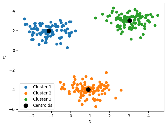
# display discovered centroids and clusters for k=3:
plt.figure()
for i in range(len(centroids)):
idx = (assignments == i)
plt.scatter(data_x[idx,0], data_x[idx,1], label=f'Cluster {i+1}')
plt.scatter(centroids[:,0], centroids[:,1], c='k', s=100, label='Centroids')
plt.xlabel(r'$x_1$')
plt.ylabel(r'$x_2$')
plt.legend()
plt.show()
Kernel Density Estimation (KDE)#
The K-means algorithm is quite useful for segmenting data into clusters, which can be useful for classifying both known and unknown data points. However, when encountering new or unseen data points it can be helpful instructive to identify new data points that lie outside the distribution of previously data points. This task is referred to as anomaly detection, and can be necessary for identifying outlier datapoints that may require special treatment or further investigation. In the materials sciences, outlier detection is crucial for identifying materials with exceptionally unique properties, or for checking that experimental data lies within the range of values predicted by some model or underlying theory.
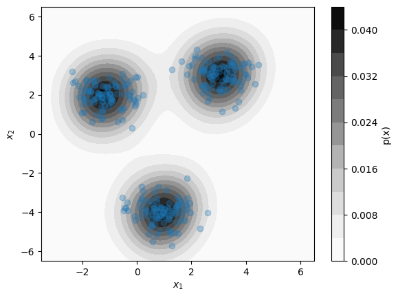
A simple way of identifying anomalous datapoints is to estimate the underlying probability distribution \(p(x)\) of known data points over the space of possible model inputs \(\mathcal{X}\). This allows for the estimation of the likelihood \(p(x')\) for some new data point \(x'\) relative to the likelihood \(p(x)\) of a previously seen datapoint \(x\). If the space of features \(\mathcal{X}\) contains continuous quantities, the underlying distribution \(p(x)\) can be straightforwardly approximated using kernel density estimation (KDE). In KDE, \(p(x)\) is estimated as an equally-weighted sum of probability distributions \(K(x)\) centered at each data point \(x_n\) with a fixed width parameter \(\alpha\):
Above, \(d\) is the dimension of \(\mathcal{X}\). A popular choice of \(K(\mathbf{x})\) is the Gaussian function:
Although KDE is relatively simple, evaluating \(p(x)\) with a naive implementation requires evaluating \(K((x-x_n)/\alpha)\) for each \(x_n\) in the dataset. More efficient implementations use data structures that avoid this linear scaling issue. A good implementation of Gaussian KDE in Python can be found in the scipy.stats.gaussian_kde module. Below, we apply this to the same dataset as above, relying on the gaussian_kde function’s automatic methods for selecting the bandwidth parameter \(\alpha\):
Show code cell source
from scipy.stats import gaussian_kde

# fit a kde model to the data:
kde = gaussian_kde(data_x.T)

# define 2D mesh grid:
x1_pts = np.linspace(-3.5,6.5,100)
x2_pts = np.linspace(-6.5,6.5,100)
x1_mesh, x2_mesh = np.meshgrid(x1_pts, x2_pts)
x_mesh = np.vstack([x1_mesh.flatten(), x2_mesh.flatten()]).T

# evaluate kde probability density on mesh points:
prob_mesh = kde(x_mesh.T).reshape(x1_mesh.shape)

# plot distribution:
plt.figure()
plt.contourf(x1_mesh, x2_mesh, prob_mesh, levels=10, cmap='Greys')
plt.colorbar(label='p(x)')
plt.scatter(data_x[:,0], data_x[:,1], label=f'Dataset', alpha=0.3)
plt.xlabel(r'$x_1$')
plt.ylabel(r'$x_2$')
plt.show()
Gaussian Mixture Model#
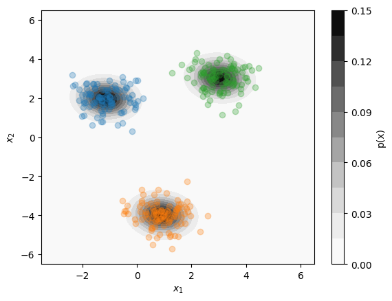
The \(k\)-means algorithm is useful for segmenting data into clusters, while KDE is useful for estimating the probability distribution of the dataset as a whole. In some cases, however, we might want to combine aspects of these two methods, such as to estimate the likelihood of a given point belonging to a specific cluster. In other words, we wish to perform both clustering and distribution estimation simultaneously. One model that can accomplish this task is the Gaussian Mixture Model. A Gaussian Mixture model can be especially useful when multiple clusters overlap in the same region of space.
Below, we give some code that uses the sklearn.mixture.GaussianMixture model to identify clusters and determine their associated probability distributions:
Show code cell source
from sklearn.mixture import GaussianMixture

# Fit a k=3 Gaussian mixture model to data:
gmm = GaussianMixture(n_components=3)
gmm.fit(data_x)

# assign points to clusters:
assignments = gmm.predict(data_x)

# define 2D mesh grid:
x1_pts = np.linspace(-3.5,6.5,100)
x2_pts = np.linspace(-6.5,6.5,100)
x1_mesh, x2_mesh = np.meshgrid(x1_pts, x2_pts)
x_mesh = np.vstack([x1_mesh.flatten(), x2_mesh.flatten()]).T

# evaluate gmm probability density on mesh points:
probs_mesh = gmm.score_samples(x_mesh).reshape(x1_mesh.shape)

# plot distribution:
plt.figure()
plt.contourf(x1_mesh, x2_mesh, np.exp(probs_mesh), levels=10, cmap='Greys')
plt.colorbar(label='p(x)')
for i in range(len(gmm.means_)):
    idx = (assignments == i)
    plt.scatter(data_x[idx,0], data_x[idx,1], label=f'Cluster {i+1}', alpha=0.3)
plt.xlabel(r'$x_1$')
plt.ylabel(r'$x_2$')
plt.show()
Exercises#
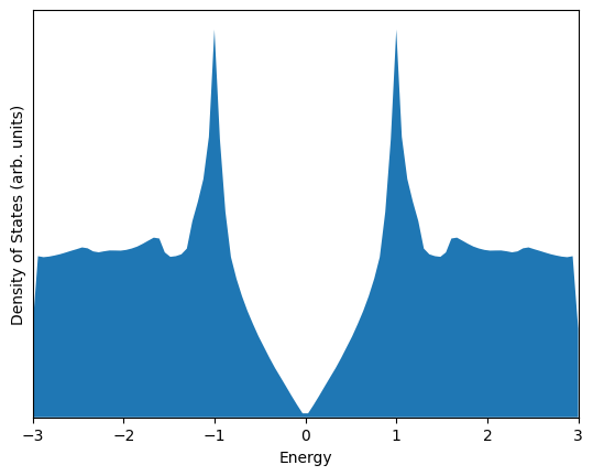
Exercise 1: Estimating Density of States with KDE
In solid state materials, electrons can occupy one of a discrete number of “allowed” energy levels; however, in periodic crystals, these energy levels are dependent on the electron wave vector \(\mathbf{k}\). This wave vector is associated with the momentum of an electron propagating in a solid.
When calculating the electronic properties of materials, a list of the “allowed” electron energies are computed for a set of uniformly sampled \(\mathbf{k}\) vectors. These energies are then combined to estimate an important distribution called the Density of States, which describes the distribution of allowed electronic states in the material with respect to the state energy.
For example, we can sample the allowed energies of the 2D material graphene using the code below:
import numpy as np

def graphene_energies(n = 100):
    rcell = np.array([[1, 0.57735], [0, 1.1547]])
    b = 2*np.pi*np.linspace(0,1,n)
    ux, uy = np.meshgrid(b,b)
    k = np.stack([ux.flatten(), uy.flatten()]).T
    k = (k @ rcell).T
    E = np.sqrt(1 + 4*np.cos(k[0]/2)**2 + 4*np.cos(k/2).prod(0))
    return np.concat((E,-E))

allowed_energies = graphene_energies()
Using the scipy.stats.gaussian_kde module, estimate and plot the density of states of graphene based on the sampled values in allowed_energies. Show the density of states from \(E = -3\) to \(E = +3\).
For optimal results, you can set the bandwidth parameter \(\alpha\) yourself by passing a float value as the parameter bw_method.
Solutions#
Exercise 1: Estimating Density of States with KDE#
Show code cell content
import matplotlib.pyplot as plt
from scipy.stats import gaussian_kde
import numpy as np

def graphene_energies(n = 100):
    rcell = np.array([[1, 0.57735], [0, 1.1547]])
    b = 2*np.pi*np.linspace(0,1,n)
    ux, uy = np.meshgrid(b,b)
    k = np.stack([ux.flatten(), uy.flatten()]).T
    k = (k @ rcell).T
    E = np.sqrt(1 + 4*np.cos(k[0]/2)**2 + 4*np.cos(k/2).prod(0))
    return np.concat((E,-E))

allowed_energies = graphene_energies()
alpha = 0.01 # This is the selected bandwidth parameter

# Estimate density of states with a Gaussian KDE
kde = gaussian_kde(allowed_energies, bw_method=alpha)
E = np.linspace(-3,3,100)
dos = kde(E)

# Plot density of states
plt.figure()
plt.fill_between(E, dos)
plt.xlim((-3, 3))
plt.ylim((0, None))
plt.xlabel('Energy')
plt.ylabel('Density of States (arb. units)')
plt.yticks([])
plt.show()