Unsupervised Learning#
Now that we have wrapped our discussion of supervised learning, let’s begin exploring unsupervised learning. Unlike supervised learning problems, which are concerned with making predictions based on labeled data, unsupervised learning problems are concerned with the identification of trends, patterns, and clusters based on unlabeled data. In supervised learning, the dataset consists of \((\mathbf{x},y)\) pairs; however in unsupervised learning, we only have the raw datapoints \(\mathbf{x}\) to work with.
As one might expect, unsupervised learning problems are generally more difficult than supervised problems. In supervised learning, where used loss functions \(\mathcal{E}(f)\) in combination with train, validation, and test sets to quantitatively measure the accuracy of proposed model. However, in unsupervised learning, there is often no clear metric that can be used to gauge the accuracy of any trends, patterns or clusters that are identified in a dataset. Often, unsupervised learning must be guided by expert intuition. As materials scientists and researchers, we supply this intuition by consulting the literature and applying known theoretical models to explain the data. When analyzing data, often we know what kinds of trends, patterns and clusters we expect to see, and we use our expert judgement to determine what kind of unsupervised learning methods are most applicable to our data.
Unsupervised Learning Methods#
There are three general categories of unsupervised learning problems that we will consider in this section:

Feature selection and dimensionality reduction
Clustering
Distribution estimation and anomaly detection
Feature Selection and Dimensionality Reduction#
In feature selection and dimensionality reduction problems, the goal is to determine which features are most meaningful in explaining how the data is distributed. This is often done in order to reduce a large set of weak data features to a small set of strong features that better describe the variance of the data. Sometimes, feature selection and dimensionality reduction are even applied prior to supervised learning tasks in order to reduce the number of features used as input to the model. This reduction in feature complexity is helpful for both visualizing data (we often have trouble visualizing data with more than three dimensions), and making models more computationally efficient. Popular methods in this category include principal components analysis (PCA), high-correlation filtering, and generalized discriminant analysis (GDA).
Clustering#
In clustering problems, the goal is to identify groupings of data points (clusters) and assign each point in the dataset to a cluster. Clustering is often used for discovering discrete classes in a dataset. It also provides an intuitive way of partitioning a large sparse dataset into smaller, denser datasets that can be analyzed individually. Popular clustering algorithms include \(k\)-means clustering, Gaussian mixture models (GMMs), and spectral clustering.
Distribution Estimation and Anomaly Detection#
In distribution estimation and anomaiy detection problems, the goal is to learn the underlying probability distribution of the data. Knowing the approximate probability distribution of data can be useful in many different circumstances, as it allows you to generate synthetic data that has the same distribution as the data, which is useful for data augmentation or Bayesian analysis. Similarly, one can use the underlying distribution of the dataset to detect anomalies (i.e. outliers) in the dataset. This is useful for problems such as disaster prediction, identification of defects, and detection of data that lies outside the training set of a model. Popular distribution estimation methods include kernel density estimation (KDE) and one-class SVMs. Some clustering techniques, such as Gaussian mixture models, can also be used for this task.
The Dimensionality of Data#
Dimensionality is an important concept in both machine learning and materials science. Much like how the dimensionality of a material’s crystal lattice plays a crucial role in the kinds of properties observed in that material, the dimensionality of a dataset plays an equally important role in what kinds of features and insights can be extracted from it. Although it is common to think of the dimensionality of a collection of datapoints as just the number of features in each point, it might be the case that if we plot the dataset, we actually find that the data is confined to some low-dimensional manifold embedded in a high-dimensional space. As an example, consider the following “Swiss Roll” manifold, which consists of a 2D plane of data that is rolled up in a 3D space:
Show code cell source
import numpy as np
import matplotlib.pyplot as plt

ax = plt.figure().add_subplot(projection='3d')

# number of points:
N = 1500

# generate "swiss roll" manifold:
theta = np.linspace(0, 3*np.pi, N)
r = theta/np.pi
x = r*np.cos(theta)
z = r*np.sin(theta)
y = np.random.uniform(0,6,N)

ax.scatter(x,y,z, alpha=0.5)
plt.title('Swiss Roll Manifold')
plt.show()
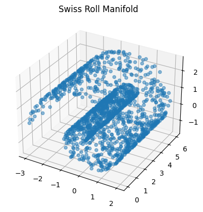
In other words, if we have a large dataset embedded in a high-dimensional space with many features, we can use dimensionality reduction techniques determine the dimensionality of the data, and ultimately “unroll” the dataset into a lower dimensional space. In the next section, we will discuss some techniques that can be applied to find these lower-dimensional representations of data.