Application: Classifying Perovskites

Application: Classifying Perovskites#

Now that we’ve covered some of the basic theory of supervised learning, let’s start applying some basic supervised learning models to a real dataset.

Perovskite Classification Dataset#

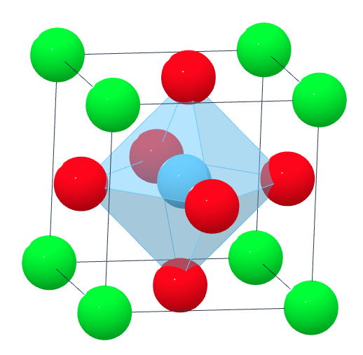
Perovskites are materials with a crystal structure of the form \(ABX_3\), where \(A\) and \(B\) are two positively charged cations and \(X\) is a negatively charged anion, usually oxygen (\(O\)). Ideal perovskites have a cubic structure, although some perovskites may attain more stable configurations with slightly perturbed structural phases, such as orthorhombic or tetragonal. Here’s an example of SrTiO\(_3\) (strontium titanate), which is most stable with a cubic structure:

We will be using the AB03 Perovskites dataset. This data was originally used in the paper Crystal structure classification in ABO3 perovskites via machine learning by Behara et al.

First, you will need to download the dataset CSV file (perovskites.csv) into the same directory as your Python notebook. You can do this by executing the following Python code in your Jupyter notebook:

import requests

CSV_URL = 'https://raw.githubusercontent.com/cburdine/materials-ml-workshop/main/MaterialsML/supervised_learning/perovskites.csv'

r = requests.get(CSV_URL)
with open('perovskites.csv', 'w') as f:
    f.write(r.text)

If the code above doesn’t work, you can also download the raw CSV file here.

Once downloaded, you can load the dataset into a pandas dataframe using the following Python code:

	Compound	A	B	In literature	v(A)	v(B)	r(AXII)(Å)	r(AVI)(Å)	r(BVI)(Å)	EN(A)	EN(B)	l(A-O)(Å)	l(B-O)(Å)	ΔENR	tG	τ	μ	Lowest distortion
0	Ac2O3	Ac	Ac	False	0	0	1.12	1.12	1.12	1.10	1.10	0.00000	0.000000	-3.248000	0.707107	-	0.800000	cubic
1	AcAgO3	Ac	Ag	False	0	0	1.12	1.12	0.95	1.10	1.93	0.00000	2.488353	-2.565071	0.758259	-	0.678571	orthorhombic
2	AcAlO3	Ac	Al	False	0	0	1.12	1.12	0.54	1.10	1.61	0.00000	1.892894	-1.846714	0.918510	-	0.385714	cubic
3	AcAsO3	Ac	As	False	0	0	1.12	1.12	0.52	1.10	2.18	0.00000	1.932227	-1.577429	0.928078	-	0.371429	orthorhombic
4	AcAuO3	Ac	Au	False	0	0	1.12	1.12	0.93	1.10	2.54	0.00000	2.313698	-2.279786	0.764768	-	0.664286	orthorhombic
...	...	...	...	...	...	...	...	...	...	...	...	...	...	...	...	...	...	...
5324	ZrWO3	Zr	W	False	1	5	0.89	0.72	0.62	1.33	2.36	2.38342	1.745600	-1.572214	0.801621	5.228952455	0.442857	cubic
5325	ZrYO3	Zr	Y	False	-	-	0.89	0.72	0.90	1.33	1.22	2.38342	2.235124	-2.489571	0.704032	-	0.642857	cubic
5326	ZrYbO3	Zr	Yb	False	-	-	0.89	0.72	0.95	1.33	1.10	2.38342	2.223981	-2.626821	0.689053	-	0.678571	orthorhombic
5327	ZrZnO3	Zr	Zn	False	-	-	0.89	0.72	0.74	1.33	1.65	2.38342	2.096141	-2.035750	0.756670	-	0.528571	cubic
5328	Zr2O3	Zr	Zr	False	-	-	0.89	0.72	0.72	1.33	1.33	2.38342	2.043778	-2.097821	0.763809	-	0.514286	cubic

5329 rows × 18 columns

Data Features#

For now, we will focus primarily on the prediction of the perovskite structure (the Lowest Distortion column). In the dataset, there are many different features given for each perovskite material. They include:

Chemical Formula (with A and B elements)
Valence of A (0-6 or unlisted): \(V(A)\)
Valence of B (0-6 or unlisted): \(V(B)\)
Radius of A at 12 coordination: \(r(A_{XII})\)
Radius of A at 6 coordination: \(r(A_{VI})\)
Radius of B at 6 coordination: \(r(B_{VI})\)
Electronegativity of A: \(EN(A)\)
Electronegativity of B: \(EN(B)\)
Bond length of A-O pair \(l(A\)-\(O)\)
Bond Length of B-O pair \(l(B\)-\(O)\)
Electronegativity difference with radius: \(\Delta ENR\)
Goldschmidt tolerance factor: \(t_G\)
New tolerance factor: \(\tau\)
Octahedral factor: \(\mu\)

In total, there are 17 distinct factors in the dataframe; however many of these features can be computed directly from other features. For example, the Goldschmidt tolarance factor is a quantity commonly used to evaluate the stability of perovskite structures. It is computed using the equation:

\[t_G = \frac{(r(A) + r(B))}{\sqrt{2}(r(B) - r(\text{O}))}\]

where \(r(A)\) and \(r(B)\) are the ionic radii of the \(A\) and \(B\) elements and \(r(\text{O})\) is the ionic radius of oxygen.

To make things a bit simpler, let’s consider only the following three factors:

Electronegativity of A: \(EN(A)\)
Electronegativity of B: \(EN(B)\)
Goldschmidt tolerance factor: \(t_G\)

We can select these features and convert them into numpy arrays using the following code:

Shape of features: (5329, 3)

Let’s also take a look at all of the distinct structures that appear in the Lowest distortion column:

['tetragonal', '-', 'cubic', 'orthorhombic', 'rhombohedral']

It appears that there are four different distinct phases listed in the dataset: rhombohedral, cubic, tetragonal, and orthorhombic. There are also some rows in the dataframe that do not have a phase listed (denoted by -). Let’s see how many of each phase are listed in the dataset:

../_images/af51e8aa40ef7106a3a751f4120843c295bf0f00d6eff46ff5333d5ba36da0b5.png

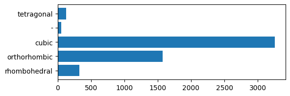
As expected, a majority of the perovskites have the ideal cubic structure.

Classifying Cubic versus Non-Cubic Structures:#

For simplicity, let’s first consider the problem of classifying cubic versus non-cubic structures. This is a simple binary classification task that we can solve using the binary perceptron model we learned about previously. Let’s start by removing the data entries with unknown structure (-) and assigning values of 1 to cubic structures and -1 to non-cubic structures:

Features shape: (5276, 3)
Binary classifier labels shape: (5329,)

Let’s visualize what the cubic versus non-cubic data looks like with respect to electronegativity (A and B):

../_images/7e60a22eb4f0063502d44aff3e7ce7d9d49d945e4070aee1a2028639c6ccf1ac.png

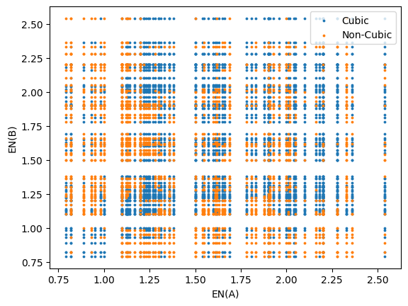
Since the electronegativity generally increases with the group and decreases with the period of elements on the periodic table, it serves as a good numerical quantity to associate with each element. This is why we observe a grid-like distribution of the data. From glancing at the distribution of cubic versus non-cubic materials, it appears that there is no immediately identifiable trend.

Let’ also look at how the cubic and non-cubic structures are distributed with respect to the Goldschmidt tolerance factor \(t_G\):

../_images/fb3e151d99e8b1882d2489ffcb3cd0958446f710a19290e222311b0a2c387615.png

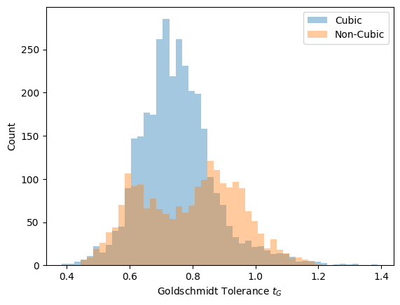
We see that a majority of the cubic structures are distributed within the range of \(t_G = 0.7\) to \(t_G = 0.9\). According to the literature, perovskites with \(t_G\) in the range of \(0.9\) to \(1.0\) are generally predicted to be in the cubic phase, which appears to be inconsistent with our data. Taking note of this discrepancy, we will proceed with preparing our data. First, we will split the data into training, validation, and test sets. This can be done with the sklearn.model_selection.train_test_split function. We will also normalize our data using sklearn.preprocessing.StandardScaler:

Shape of z_train: (4263, 3)
Shape of z_val: (533, 3)
Shape of z_test: (533, 3)

The Perceptron (Linear Classification) Model#

One of the simplest two-class classification models is a linear classifier model, historically referred to as a Perceptron model. For a normalized feature vector \(\mathbf{z}\) with \(N\) features, a linear classifier model \(f(\mathbf{z})\) makes “1” and “-1” class predictions according to the equation:

\[\begin{split}f(\mathbf{z}) = \begin{cases} 1, & w_0 + \sum_{i=1}^N w_iz_i > 0 \\ -1, & \text{ otherwise} \end{cases}\end{split}\]

where \(w_0, w_1, ..., w_N\) are learned weights of the model. In this case, a prediction of \(1\) corresponds to the cubic class, and \(-1\) corresponds to the non-cubic class. We can fit a Perceptron model to the data using the sklearn.linear_model.Perceptron class.

training set accuracy:   0.6328876378137462
validation set accuracy: 0.6135084427767354

From our visualization of the cubic vs. non-cubic perovskites, we saw that the separation between these two classes is very non-linear, so we expect both the training set and validation accuracy to be low. Nonetheless, we do see that the validation accuracy is greater than \(0.6\), which appears to be statistically significant improvement upon random guessing.

The Nearest Neighbor Model#

Before trying other models, it may help to see what kind of accuracy can be attained by a nearest neighbor classification model. As the name suggests, a nearest neighbor classification model predicts the class of an unseen normalized data point \(\mathbf{z}\) to be the majority class in the set of \(k\) normalized data points in the training set that are nearest to \(\mathbf{z}\). By “nearest”, we refer to the point with the smallest Euclidean distance:

\[d(\mathbf{z},\mathbf{z}') = \lVert \mathbf{z} - \mathbf{z}' \rVert\]

Typically, an odd number of neighbors \(k\) is used. While \(k\)-nearest neighbor models tend to give good results, they may not be suitable for large datasets or datasets with many features, as searching for the nearest neighbors in a dataset may be computationally expensive.

training set accuracy:   0.8184377199155525
validation set accuracy: 0.7729831144465291

An important property of nearest neighbor models is that no learning actually takes place with the training data; rather, the model is the training data. This can be viewed as either a criticism or a strength of the model, depending on whether the goal is to just to make accurate predictions or to find a simple and interpretable model that still makes accurate predictions. Often the latter kind of model is preferred over the former, so nearest neighbor models are not often the best choice for supervised tasks. However, these models can be useful in establishing a baseline accuracy that one can attempt to match with models that have less complexity.

As expected, the nearest neighbor model is much more accurate than the Perceptron model we tried earlier. This is because it is capable of capturing some of the non-linearities of classes, especially with regards to the electronegativity of the \(A\) and \(B\) atoms. We can write some Python code to visualize this as follows:

../_images/f2006f9db730acab3e9fac56ba80624e5ec952a5ca0012ba4737636c4b7bad08.png

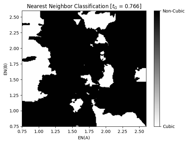
Now that we have established a baseline accuracy using the nearest neighbor model, let’s try to exceed this baseline accuracy with a more complex model.

Decision Tree Classifier#

Next, let’s try a model that is slightly more complex than the perceptron classifier: a Decision Tree Classifier. As the name suggests, a decision tree classifier works by constructing a decision tree based on individual features. Decision trees are especially well-suited to datasets with independent features that tend to exist in many small clusters. Since the distribution of cubic and non-cubic perovskites with respect to electronegativity is grid-like and contains many small clusters, we may obtain good results with a decision tree. To fit a decision tree to the data, we will use the sklearn.tree.DecisionTreeClassifier model. Since most of the sklearn models conform to the same interface for fitting and evaluating model accuracy, we only need to make a few changes to our code to try out this model:

training set accuracy:   0.8688716866056767
validation set accuracy: 0.7842401500938087

Comparing the validation error of the decision tree classifier with the nearest neighbor model from before, we see that the decision tree classifier performs slightly better.

Application: Classifying Perovskites

Contents