Application: Classifying Superconductors#
Now that we have a strong understanding of unsupervised learning, let’s apply what we have learned to study a class of materials known as superconductors. Superconductors are materials that exhibit zero electrical resistance below a critical temperature \(T_c\). These materials also exhibit the Meissner Effect, meaning they expel magnetic fields within the bulk of the material. This facilitates stable magnetic levitation at temperatures below \(T_c\).

Understanding patterns in superconductors’ compositions and external conditions (such as pressure applied to the material) can help identify trends that correlate with desired high-\(T_c\) behavior. These insights could be leveraged to discover new kinds of superconductors or to help engineer the external conditions needed to raise the \(T_c\) of known superconductors.
You can download the dataset for this section using the following Python code:
import requests

CSV_URL = 'https://raw.githubusercontent.com/cburdine/materials-ml-workshop/main/MaterialsML/unsupervised_learning/matml_supercon_cleaned.csv'

r = requests.get(CSV_URL)
with open('matml_supercon_cleaned.csv', 'w', encoding='utf-8') as f:
    f.write(r.text)
Alternatively, you can download the CSV file directly here.
Loading the Dataset#
Let’s begin by loading the dataset in to a Pandas dataframe and then perform some basic data cleaning. Specifically, we will remove entries with missing compositions and those with anomalously high \(T_c\) values (likely errors or non-physical outliers). We then display the dataset to view the data features:
Show code cell source
import pandas as pd

# load dataset into a pandas DataFrame:
SUPERCON_CSV = 'matml_supercon_cleaned.csv'
data_df = pd.read_csv(SUPERCON_CSV)

# remove rows for materials with an ambiguous composition:
data_df = data_df[data_df['Composition'].isnull() == False]

# remove corrupted data with invalid Tc:
data_df = data_df[data_df['Tc (K)'] < 400]

# show dataframe in notebook:
display(data_df)
| Material | Substitutions | Composition | Tc (K) | Pressure (GPa) | Shape | Substrate | DOI | |
|---|---|---|---|---|---|---|---|---|
| 1 | In O | {} | {'In': 1, 'O': 1} | 2.00 | 0.0 | films | NaN | 10.1134/1.568304 |
| 2 | Pr Ru 2 Si 2 | {} | {'Pr': 1, 'Ru': 2, 'Si': 2} | 14.00 | 0.0 | NaN | NaN | 10.1088/0953-8984/12/34/307 |
| 3 | Lu 3 Os 4 Ge 13 | {} | {'Lu': 3, 'Os': 4, 'Ge': 13} | 2.85 | 0.0 | NaN | NaN | NaN |
| 4 | La Mn O 3.04 | {} | {'La': 1, 'Mn': 1, 'O': 3.04} | 125.00 | 0.0 | NaN | NaN | 10.1103/physrevlett.87.127206 |
| 5 | La Mn O 3.045 | {} | {'La': 1, 'Mn': 1, 'O': 3.045} | 130.00 | 0.0 | NaN | NaN | 10.1103/physrevlett.87.127206 |
| ... | ... | ... | ... | ... | ... | ... | ... | ... |
| 23876 | Nb Se 2 | {} | {'Nb': 1, 'Se': 2} | 7.00 | 0.0 | nanobelts | NaN | 10.1103/physrevb.75.020501 |
| 23877 | Mg B 2 | {} | {'Mg': 1, 'B': 2} | 40.00 | 0.0 | NaN | NaN | 10.1103/physrevb.66.012511 |
| 23878 | Ca Bi 2 | {} | {'Ca': 1, 'Bi': 2} | 2.00 | 0.0 | NaN | NaN | NaN |
| 23879 | Ca Bi 2 | {} | {'Ca': 1, 'Bi': 2} | 2.00 | 0.0 | single-crystalline | NaN | NaN |
| 23880 | Cd 2 Re 2 O 7 | {} | {'Cd': 2, 'Re': 2, 'O': 7} | 1.00 | 0.0 | single crystals | NaN | 10.1016/s0022-3697(02)00090-2 |
19463 rows × 8 columns
Here’s a summary of the different features included in the dataset:
Material: The chemical formula of the superconducting material.
Substitutions: Python dictionary consisting of doping ratios.
Composition: Composition of the chemical formula under doping.
Tc: Reported critical temperature of superconductivity (K).
Pressure: Applied pressure to superconducting sample (GPa).
Shape: Shape of the superconducting sample (if any).
Substrate: Substrate the sample was deposited on (if any).
DOI: DOI of paper that data was extracted from.
In this section, we will not attempt to predict any superconductor properties; instead, we will aim to extract insight from this dataset by applying clustering and distribution estimation models.
Preprocessing Data#
Machine learning models require numerical inputs, so we will need to convert the materials’ compositions (stored as Python dictionaries in string form) into fixed-length feature vectors. First, we will normalize the elemental compositions to account for different formula unit sizes. We will also append the applied pressure and \(T_c\) to each feature vector. Finally, we will standardize the data to have zero mean and unit variance—a common preprocessing step for most ML algorithms.
To simplify the data conversion process, we will create a set ELEMENTS that contains all elements
appearing in the dataset. We will also create a function called vectorize_composition() that will convert each chemical composition dictionary into a minimal feature vector:
Show code cell source
import numpy as np
import ast

# Generate a list of elements in the dataset:
ELEMENTS = set()
for v in data_df['Composition'].values:
    ELEMENTS |= set(ast.literal_eval(v).keys())
ELEMENTS = sorted(ELEMENTS)

def vectorize_composition(composition, elements):
    """ converts an elemental composition dict to a vector. """
    total_n = sum(composition.values())
    vec = np.zeros(len(elements))
    for elem, n in composition.items():
        if elem in elements:
            vec[elements.index(elem)] = n/total_n
    return vec

print('Number of elements:', len(ELEMENTS))
Number of elements: 86
Now that we can convert the chemical composition of each material into a feature vector, we will write another function that parses each row in the DataFrame:
import ast

def parse_data_vector(row):
    """ parses data from a dataframe row """

    # parse the composition dict:
    composition_dict = ast.literal_eval(row['Composition'])

    # parse feature vector (x):
    x_vector = np.concatenate([
        vectorize_composition(composition_dict, ELEMENTS),
        np.array([ row['Pressure (GPa)'] ]),
        np.array([ row['Tc (K)'] ]),
    ])

    return x_vector
Finally, we parse each row of the DataFrame with parse_data_row() and standardize the data with StandardScaler:
from sklearn.preprocessing import StandardScaler

data_x = np.array([
    parse_data_vector(row)
    for _, row in data_df.iterrows()
])

print(data_x.shape)

# standardize data:
scaler = StandardScaler()
data_z = scaler.fit_transform(data_x)

# extract a matrix of only compositions:
composition_z = data_z[:,:-2]
(19463, 88)
Estimate the Empirical Distribution of \(T_c\)#
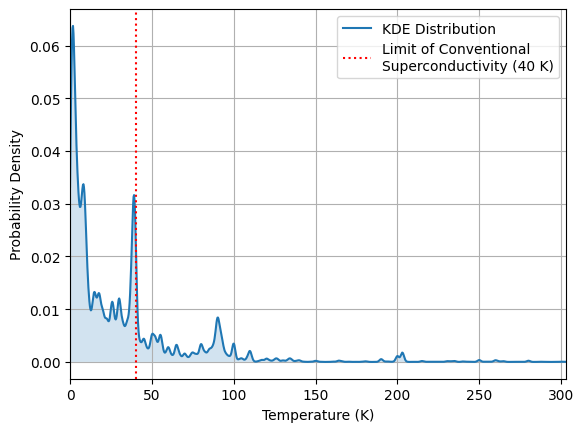
To understand how \(T_c\) values are distributed among the known superconductors in our dataset, we will use kernel density estimation (KDE). This non-parametric method lets us estimate a smooth probability density function with respect to \(T_c\). Instead of using the basic KDE module in scipy.stats, we will use the more advanced module that is available in sklearn.neighbors.KernelDensity:
from sklearn.neighbors import KernelDensity

Tc_data = data_x[:,-1]
Tc_kde = KernelDensity(kernel='gaussian').fit(Tc_data.reshape(-1,1))
Let’s visualize the distribution, and inspect how the \(T_c\) values are distributed. Since 40 K is believed to be the limit of low-temperature conventional superconductivity, let’s see how the data is distributed around this point:
import matplotlib.pyplot as plt

# generate points to evaluate the KDE model:
Tc_eval_pts = np.linspace(0, np.max(Tc_data), 1000)

# determine the standardized density of the distribution:
Tc_density = np.exp(Tc_kde.score_samples(
                        Tc_eval_pts.reshape(-1,1)))
Tc_density /= np.trapz(Tc_density, Tc_eval_pts)

plt.figure()
plt.plot(Tc_eval_pts, Tc_density, label='KDE Distribution')
plt.fill_between(Tc_eval_pts, Tc_density, alpha=0.2)
plt.axvline(
    40,  linestyle=':', color='r',
    label='Limit of Conventional\nSuperconductivity (40 K)')
plt.grid()
plt.xlabel('Temperature (K)')
plt.ylabel('Probability Density')
plt.legend()
plt.xlim(0,np.max(Tc_data))
plt.show()
Show code cell output
/tmp/ipykernel_69810/1067493337.py:9: DeprecationWarning: `trapz` is deprecated. Use `trapezoid` instead, or one of the numerical integration functions in `scipy.integrate`.
  Tc_density /= np.trapz(Tc_density, Tc_eval_pts)
Identifying Outliers in the Distribution:#
Materials with extremely high or low \(T_c\) values may represent outliers or materials that exhibit unique physical properties. Let’s take a look at any outlying data points by identifying the least probable data points (i.e., the lowest log-likelihood under the KDE model). These can be studied further to see if they reveal special physics or data issues.
To score the log-likelihood of each data point, we use the score_samples() function and select the \(N = 10\) points that have the least likelihood:
N_outliers = 10

log_likelihoods = Tc_kde.score_samples(Tc_data.reshape(-1,1))
cutoff = np.sort(log_likelihoods)[N_outliers]

outlier_df = data_df[log_likelihoods < cutoff]
display(outlier_df[['Material','Tc (K)','Pressure (GPa)','DOI']])
| Material | Tc (K) | Pressure (GPa) | DOI | |
|---|---|---|---|---|
| 520 | Y H 6 | 290.0 | 300.0 | 10.1103/physrevb.99.220502 |
| 618 | Si 2 H 6 | 153.0 | 170.0 | NaN |
| 1422 | Sc H 6 | 196.0 | 170.0 | 10.1007/1-4020-3989-1_6 |
| 2879 | H 3 S 0.96 Si 0.04 | 274.0 | 170.0 | NaN |
| 3714 | Y H 10 | 303.0 | 400.0 | NaN |
| 4164 | Y H 9 | 256.0 | 177.0 | NaN |
| 6699 | K H 2 P O 4 | 210.0 | 170.0 | NaN |
| 10629 | Si 2 H 6 | 174.0 | 275.0 | 10.1016/j.physc.2012.12.002 |
| 14301 | H 3 S | 178.0 | 170.0 | 10.1038/srep38570 |
| 20021 | La H 10 | 218.0 | 170.0 | NaN |
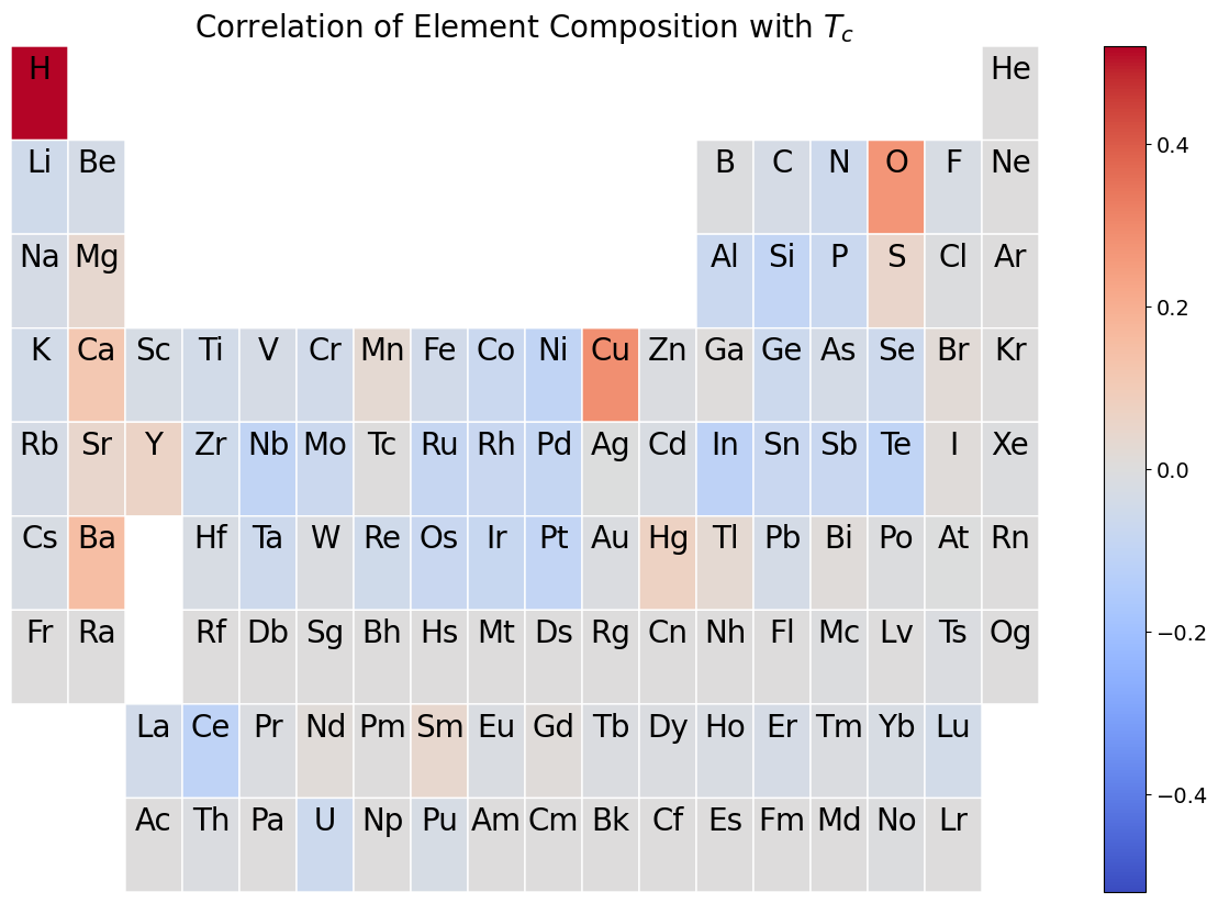
Correlations of Composition with \(T_c\)#
To explore which elements are most strongly associated with superconductivity, we will compute the covariance between each compositional feature and the standardized \(T_c\). A heatmap on the periodic table then visually shows which elements are associated with increases or decreases in the critical temperature when they are added to a material.
First, we compute the covariance matrix of the data and extract the column corresponding to the \(T_c\) of each material:
cov_matrix = np.cov(data_z.T)
Tc_covs = cov_matrix[:-2,-1]
Next, we visualize the results using the periodic_table_heatmap() function from Pymatgen.
from pymatgen.util.plotting import periodic_table_heatmap

import matplotlib.pyplot as plt
import matplotlib
# convert Tc covariances to an (element -> cov.) dictionary:
Tc_element_covs = {
    elem : cov
    for elem, cov in zip(ELEMENTS, Tc_covs)
}

# plot covariance periodic table heatmap:
max_cov = np.max(np.abs(Tc_covs))
heatmap = periodic_table_heatmap(
    Tc_element_covs,
    cmap='coolwarm',
    symbol_fontsize=20,
    cmap_range=(-max_cov, max_cov),
    blank_color=matplotlib.colormaps['coolwarm'](0.5)
)
plt.title('Correlation of Element Composition with $T_c$', fontsize='20')
plt.show()
Show code cell output
You're using a deprecated version of periodic_table_heatmap(). Consider `pip install pymatviz` which offers an interactive plotly periodic table heatmap. You can keep calling this same function from pymatgen. Some of the arguments have changed which you'll be warned about. To disable this warning, pass pymatviz=False.
Identifying Clusters in the Data#
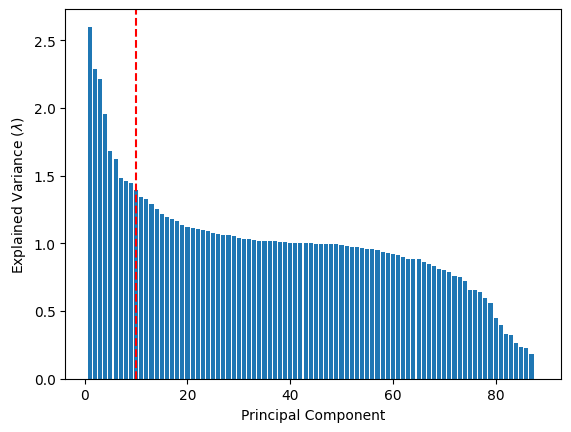
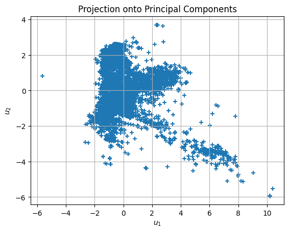
As we have learned in the previous section, dimensionality reduction techniques like PCA allow us to summarize high-dimensional data using a smaller number of principal components. We project the data into this reduced space and then use k-means clustering to group similar superconductors together. These clusters may reflect different material families or classes of superconductors.
from sklearn.decomposition import PCA

full_pca = PCA(n_components=data_z.shape[1])
full_pca.fit(data_z)
lambdas = full_pca.explained_variance_
# cutoff (selected by inspecting the plot below)
pca_cutoff = 10
Show code cell source
# plot explained variance vs. principal component:
plt.figure()
plt.bar(np.arange(1,len(lambdas)+1),lambdas)
plt.ylabel(r'Explained Variance ($\lambda$)')
plt.axvline(pca_cutoff, linestyle='--', color='r',
            label=f'Selected Cutoff: {pca_cutoff}')
plt.xlabel('Principal Component')
plt.show()
pca = PCA(n_components=pca_cutoff)
data_u = pca.fit_transform(data_z)

plt.figure()
plt.grid()
plt.scatter(data_u[:,0], data_u[:,1], marker='+')
plt.xlabel(r'$u_1$')
plt.ylabel(r'$u_2$')
plt.title('Projection onto Principal Components')
plt.show()
Show code cell output
from sklearn.cluster import KMeans

# number of clusters to find:
n_clusters = 6
kmeans = KMeans(n_clusters, n_init='auto')
kmeans.fit(data_u)
assignments = kmeans.predict(data_u)

clusters = {}
for i in range(n_clusters):
    clusters[i] = data_u[assignments == i]
Show code cell source
plt.figure()
for i, cluster in clusters.items():
   plt.scatter(cluster[:,0], cluster[:,1], marker='+',
               label=f'Cluster {i}')
plt.xlabel(r'$u_1$')
plt.ylabel(r'$u_2$')
plt.title('Principal Component Clusters')
plt.legend()
plt.show()
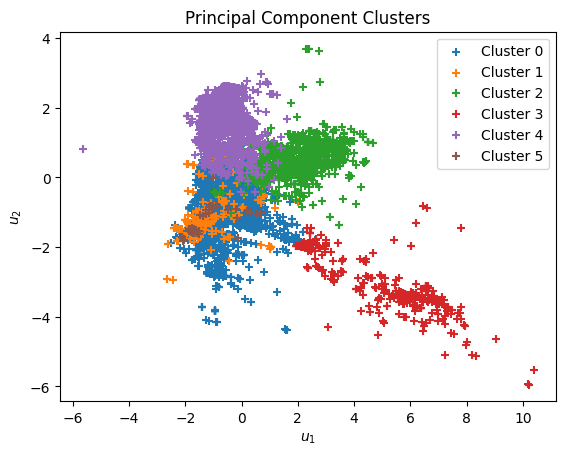
To interpret the clusters, we display representative samples from each. You might notice that some clusters are enriched in certain elements or tend to have higher or lower \(T_c\). These clusters could guide targeted exploration in materials discovery:
Show code cell content
# show some samples of each cluster:
for i in clusters.keys():

    # obtain cluster dataframe:
    cluster_df = data_df[assignments == i]
    sample_df = cluster_df[
        ['Material', 'Tc (K)', 'Pressure (GPa)', 'DOI']
    ].sample(5)

    # show sample dataframe:
    display(f'Cluster {i} Examples:')
    display(sample_df)
'Cluster 0 Examples:'
| Material | Tc (K) | Pressure (GPa) | DOI | |
|---|---|---|---|---|
| 18630 | Nb 2 Pd 0.81 S 5 | 6.60 | 0.0 | 10.1103/physrevb.98.014502 |
| 2647 | La Pt 3 Si | 0.60 | 0.0 | 10.1143/jpsj.78.014705 |
| 8325 | Bi | 0.53 | 0.0 | 10.1126/science.aaf8227 |
| 4983 | Y Ni 2 B 2 C | 15.50 | 0.0 | 10.1142/s0217979200002983 |
| 8755 | Nb C | 12.00 | 0.0 | 10.1002/3527600434.eap790 |
'Cluster 1 Examples:'
| Material | Tc (K) | Pressure (GPa) | DOI | |
|---|---|---|---|---|
| 7736 | Ce Ir In 5 | 0.4 | 0.0 | 10.1103/physrevb.85.060505 |
| 2970 | Ce O Bi S 2 | 1.3 | 0.0 | NaN |
| 17613 | In | 3.4 | 0.0 | 10.1140/epjb/e2005-00158-7 |
| 13159 | Ce Co In 5 | 2.3 | 0.0 | 10.1103/physrevlett.114.027003 |
| 8735 | Ce Cu 2 Si 2 | 1.5 | 0.0 | 10.1002/3527600434.eap790 |
'Cluster 2 Examples:'
| Material | Tc (K) | Pressure (GPa) | DOI | |
|---|---|---|---|---|
| 7982 | La 1-x Ca x Mn O 3 | 17.7 | 0.0 | 10.1103/physrevb.65.104419 |
| 1479 | Bi 2 Sr 2 Ca Cu 2 O 8 | 74.0 | 0.0 | 10.1103/physrevb.81.224518 |
| 19379 | Y Ba 2 Cu 3 O 6.95 | 93.0 | 0.0 | 10.1038/nature04704 |
| 13651 | Bi 2 Sr 2 Ca Cu 2 O 8 | 83.0 | 0.0 | 10.1103/physrevb.77.054520 |
| 2102 | Sr 2 Ru O 4 | 1.0 | 0.0 | 10.1134/s1063776114060132 |
'Cluster 3 Examples:'
| Material | Tc (K) | Pressure (GPa) | DOI | |
|---|---|---|---|---|
| 16536 | Sn H 14 | 97.0 | 300.0 | 10.1103/physrevb.99.024508 |
| 14268 | H 2 S | 200.0 | 200.0 | 10.1103/physrevb.93.094525 |
| 625 | Al H 3 | 7.0 | 125.0 | NaN |
| 3716 | Mg H 6 | 271.0 | 300.0 | NaN |
| 6773 | Se H 3 | 100.0 | 0.0 | 10.1103/physrevb.92.060508 |
'Cluster 4 Examples:'
| Material | Tc (K) | Pressure (GPa) | DOI | |
|---|---|---|---|---|
| 5781 | Ba (Fe 0.9 Co 0.1) 2 As 2 | 19.5 | 0.0 | 10.1016/j.physb.2012.01.021 |
| 2820 | Rb Fe 2 As 2 | 2.1 | 0.0 | 10.1103/physrevb.91.024502 |
| 4418 | K Ca 2 Fe 4 As 4 F 2 | 28.2 | 0.0 | 10.1103/physrevmaterials.1.044804 |
| 8980 | Ba Fe 2 As 2 | 24.0 | 0.0 | NaN |
| 9371 | Ba Fe 2 As 2 | 12.0 | 0.0 | NaN |
'Cluster 5 Examples:'
| Material | Tc (K) | Pressure (GPa) | DOI | |
|---|---|---|---|---|
| 21791 | Pu Co Ga 5 | 18.6 | 0.0 | 10.1016/j.jallcom.2018.02.116 |
| 9143 | Pu Co Ga 5 | 18.5 | 0.0 | 10.1088/0953-8984/23/34/349501 |
| 11196 | Mo 6 Ga 31 | 8.0 | 0.0 | 10.1038/s41598-019-49846-y |
| 22896 | Ir 2 Ga 9 | 2.2 | 0.0 | 10.1143/jpsj.76.073708 |
| 2424 | Pu Co Ga 5 | 18.5 | 0.0 | 10.1016/j.physb.2005.11.047 |