Advanced Regression Models

In the last section, we learned about how regression models can be fit to data using the gradient descent learning algorithm. Interestingly, for certain regression models, the optimal “best fit” solution can be found in closed form. The simplest of these closed-form models is multivariate linear regression.

Multivariate Linear Regression

At the name suggests, multivariate linear regression models are generalizations of linear regression models where \(\mathbf{x}\) has many dimensions. A linear regression model for a \(D\)-dimensional feature vector \(\mathbf{x}\) takes the form:

\[\hat{y} = f(\mathbf{x}) = w_0 + \sum_{i=1}^D w_ix_i\]

where \(w_0\) and the \(w_i\) are the weights that must be learned. If we define \(\underline{\mathbf{x}} = \begin{bmatrix} 1 & x_1 & x_2 & ... & x_D \end{bmatrix}^T\) (the vector \(\mathbf{x}\) prepended with \(1\)), we can write \(f(x)\) as an inner product of \(\underline{\mathbf{x}}\) with the weight vector \(\mathbf{w} = \begin{bmatrix} w_0 & w_1 & w_2 & ... & w_D \end{bmatrix}^T\):

\[\hat{y} = f(\mathbf{x}) = \underline{\mathbf{x}}^T\mathbf{w}\]

For linear regression models, it is helpful to represent a dataset \(\{ (\mathbf{x}_n,y_n) \}_{n=1}^N\) as a matrix-vector pair \((\mathbf{X},\mathbf{y})\), given by:

\[\begin{split}\mathbf{X} = \begin{bmatrix} \underline{\mathbf{x}_1}^T \\ \underline{\mathbf{x}_2}^T \\ \vdots \\ \underline{\mathbf{x}_N}^T \end{bmatrix},\qquad\qquad \mathbf{y} = \begin{bmatrix} y_1 \\ y_2 \\ \vdots \\ y_N \end{bmatrix}\end{split}\]

In terms of \(\mathbf{X}\) and \(\mathbf{y}\), the task of fitting the linear regression model reduces to solving the weights \(\mathbf{w}\) satisfying the matrix equation \(\mathbf{X}\mathbf{w} \approx \mathbf{y}\). Since most datasets have some degree of noise, it is usually impossible to find a weight vector \(\mathbf{w}\) for which \(\mathbf{X}\mathbf{w} = \mathbf{y}\) exactly. Instead, we must settle for weights \(\mathbf{w}\) that minimizes a some loss function. The most popular choice of loss function for linear regression is the mean square error (MSE). In terms of \(\mathbf{X}\) and \(\mathbf{y}\), the MSE can be written as:

\[\mathcal{E}(f) = \frac{1}{N}(\mathbf{X}\mathbf{w} -\mathbf{y})^T(\mathbf{X}\mathbf{w} - \mathbf{y})\]

It can be shown that the weights \(\mathbf{w}\) minimizing \(\mathcal{E}(f)\) can be computed in closed form as \(\mathbf{w} = \mathbf{X}^+\mathbf{y}\), where \(\mathbf{X}^+\) is the Moore-Penrose inverse (sometimes called the pseudo-inverse) of \(\mathbf{X}\). For a sufficiently well-conditioned data matrix \(\mathbf{X}\), the weights can be computed as:

\[\mathbf{w} = \mathbf{X}^{+}\mathbf{y} = \left( (\mathbf{X}^T\mathbf{X})^{-1}\mathbf{X}^T\right)\mathbf{y}\]

For most applications, fitting linear regression models with the Moore-Penrose inverse is preferred to other methods, such as gradient descent.

Tip

To compute the Moore-Penrose inverse in Python, you can use the np.linalg.pinv function.

High-Dimensional Embeddings

While linear regression models are quite powerful and admit and optimal closed-form fit, they often fail to yield good predictions on data with non-linear trends. Fortunately, we can extend the closed form solution of linear regression to work with some non-linear models as well. The general idea behind this extension is to embed the feature vector \(\mathbf{x}\) into a high-dimensional space where linear regression can be applied. Often, this embedding is a non-linear function of \(\mathbf{x}\), which allows for the model to perform regression based on non-linear functions of the features \(\mathbf{x}\). These embedding models have the general form:

\[ f(\mathbf{x}) = w_0 + \sum_{j=1}^{D_{emb}} w_j \phi_j(\mathbf{x})\]

where the \(\phi_j: \mathbb{R}^{D} \rightarrow \mathbb{R}\) are the embedding functions and \(D_{emb}\) is the dimension of the embedding. In most cases, \(D_{emb} > D\). As with standard multivariate linear regression, the MSE loss is commonly used. The MSE loss of the embedding model is:

\[\mathcal{E}(f) = \frac{1}{N}(\mathbf{\Phi}(\mathbf{X})\mathbf{w} - \mathbf{y})^T(\mathbf{\Phi}(\mathbf{X})\mathbf{w} - \mathbf{y})\]

where \(\mathbf{\Phi}(\mathbf{X})\) is the embedding of the data matrix \(\mathbf{X}\):

\[\begin{split}\mathbf{\Phi}(\mathbf{X}) = \begin{bmatrix} 1 & \phi_1(\mathbf{x}_1) & \phi_2(\mathbf{x}_1) & \dots & \phi_{D_{emb}}(\mathbf{x}_1) \\ 1 & \phi_1(\mathbf{x}_2) & \phi_2(\mathbf{x}_2) & \dots & \phi_{D_{emb}}(\mathbf{x}_2) \\ \vdots & \vdots & \vdots & \ddots & \vdots \\ 1 & \phi_1(\mathbf{x}_N) & \phi_2(\mathbf{x}_N) & \dots & \phi_{D_{emb}}(\mathbf{x}_N) \end{bmatrix}\end{split}\]

The MSE-minimizing weight vector \(\mathbf{w}\) can be solved for using the Moore-Penrose inverse: \(\mathbf{w} = \mathbf{\Phi}(\mathbf{X})^{+}\mathbf{y}\).

Example: Polynomial Fits of Single-Variable Functions

We have already studied the problem of fitting a polynomial of degree \(D\) to a single-variable \(\mathbf{x}\) with gradient descent. It turns out that we can actually obtain a closed-form best fit using the method of high-dimensional embeddings, where the \(\phi_j\) functions are simply powers of \(\mathbf{x}\): \(\phi_j(\mathbf{x}) = x^j\) (Since \(\mathbf{x}\) is a vector of length 1, we can treat \(\mathbf{x}\) as a scalar \(x\)). The embedding matrix \(\mathbf{\Phi}(\mathbf{X})\) for a polynomial model is known as a Vandermonde matrix:

\[\begin{split}\mathbf{\Phi}(\mathbf{X}) = \begin{bmatrix} 1 & x_1 & x_1^2 & \dots & x_1^{D_{emb}} \\ 1 & x_2 & x_2^2 & \dots & x_2^{D_{emb}} \\ 1 & x_3 & x_3^2 & \dots & x_3^{D_{emb}} \\ \vdots & \vdots & \vdots & \ddots & \vdots \\ 1 & x_N & x_N^2 & \dots & x_N^{D_{emb}} \end{bmatrix}\end{split}\]

One can easily compute the optimal weights \(\mathbf{w}\) of a degree \(D_{emb}\) polynomial fit by computing the Moore-Penrose inverse of this matrix. In fact, this is the method used in the np.polyfit function, which we have used before.

Underfitting and Overfitting

One of the benefits of using high-dimensional embeddings of data is that it allows for many different possible non-linear functions to be incorporated into the model \(f(\mathbf{x})\), allowing for a high model flexibility. This flexibility, however, can come at a significant cost: the more weights a model has, the more likely it is to overfit the data. What do we mean by overfitting? Overfitting occurs when the predictions made by a fitted model correspond too closely to the training data and therefore fail to correspond to unseen data not contained in the training dataset. Put simply, overfitted models tend to “memorize” the training data instead of “learn” from it.

If a model is too inflexible, it may be subject to the opposite problem: underfitting. Underfitting occurs when the model is unable to capture the underlying trends of the data. Typically, underfitting occurs as a result of poor model choice. A good model is one that strikes a balance between these extremes, being just flexible enough to learn the underlying trends of the training data, but not so flexible that it simply “memorizes” the training data.

To help illustrate underfitting and overfitting, let’s return to the familiar example of fitting 1D data with polynomials:

Show code cell source Hide code cell source

import numpy as np
import matplotlib.pyplot as plt

# seed random number generator:
np.random.seed(0)

# define data distribution:
def y_distribution(x):
	return -0.1*(x-5)**2 + 1.0 + \
            np.random.normal(0,0.3,size=len(x))

# generate training data:
data_n = 12
data_x = np.linspace(0,10,data_n)
data_y = y_distribution(data_x)

# fit data to a line (degree 1 polynomial):
xy_linefit = np.poly1d(np.polyfit(data_x,data_y,deg=1))

# fit data to a quadratic (degree 2 polynomial):
xy_quadfit = np.poly1d(np.polyfit(data_x,data_y,deg=2))

# fit data to N-1 degree polynomial to data:
xy_polyfit = np.poly1d(np.polyfit(data_x,data_y,deg=data_n-1))

# plot data and models for comparison:
plt.figure()
eval_x = np.linspace(0,10,1000)
plt.scatter(data_x,data_y, color='k', label=r'Training Data $(x,y)$')
plt.plot(eval_x, xy_linefit(eval_x), label=r'Linear Fit ($D_{emb} = 1$)')
plt.plot(eval_x, xy_quadfit(eval_x), label=r'Quadratic Fit ($D_{emb} = 2$)')
plt.plot(eval_x, xy_polyfit(eval_x), 
         label=r'Polynomial Fit ($D_{emb} = ' + f'{data_n-1}' + '$)')
plt.xlabel('x')
plt.ylabel('y')
plt.legend()
plt.show()

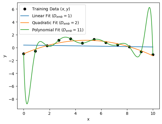
In the plot above, the polynomial with \(D_{emb} = 11\) fits the data perfectly; however, we can see that it interpolates between data points very poorly, especially at the edges of the data distribution, where \(x \approx 0\) and \(x \approx 10\). It is very likely that this model is overfitting the data. On the other hand, we see that the linear model (\(D_{emb} = 1\)) is not flexible enough to capture the non-linearities of the data. As a result, it is very likely that this model is underfitting the data. The quadratic fit (\(D_{emb} = 2\)) seems to neither overfit nor underfit the data, which suggests it is the best model for this training dataset.

Identifying Overfitting

The easiest way of identifying is a model is overfitting the data is by comparing the error of the model on the training and validation error. Since the model is only fit to the training set data, the validation set error gives us an idea of how accurate the model is on unseen data. If the validation error is significantly higher than the training error and the training error is close to its minimum, the model is likely overfitting the data. On the other hand, if both the training and validation error are high, the model is likely underfitting the data.

To illustrate this, we plot the training and validation error of our 1D polynomial models and indicate the regions of overfitting and underfitting:

Show code cell source Hide code cell source

# validation dataset (for the sake of illustration):
val_data_x = np.linspace(-1,11, 5)
val_data_y = y_distribution(val_data_x)

# embedding dimensions to try:
embedding_dims = list(range(1, 8))

# initialize lists to store results:
models = []
train_errors = []
validation_errors = []

for d in embedding_dims:

    # fit the model to the training set:
    xy_fit = np.poly1d(np.polyfit(data_x, data_y, deg=d))
    
    # compute mean square error for training and validation set:
    train_error = np.mean((xy_fit(data_x) - data_y)**2)
    validation_error = np.mean((xy_fit(val_data_x) - val_data_y)**2)

    # record results:
    models.append(xy_fit)
    train_errors.append(train_error)
    validation_errors.append(validation_error)

# identify regions of under/overfitting:
underfit_region = (0.5, 1.5)
overfit_region = (5.5,7.5)

# plot train/validation error versus embedding dimension curve:
plt.figure(figsize=(6.5,2))
plt.plot(embedding_dims, train_errors, 'o:', label='Training Set Error')
plt.plot(embedding_dims, validation_errors, 'o:', label='Validation Set Error')
plt.ylim((-0.2,6.0))
plt.xlim((min(underfit_region),max(overfit_region)))
plt.xlabel('Polynomial Degree ($D_{emb}$)')
plt.ylabel('$\mathcal{E}(f)$ (Mean Square Eror)')
plt.axvspan(*underfit_region, alpha=0.4, color='orange', label='Underfitting')
plt.axvspan(*overfit_region, alpha=0.3, color='red', label='Overfitting')
plt.legend()
plt.show()

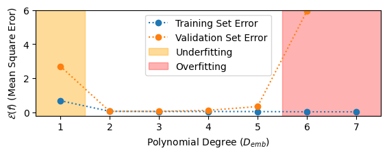
We can see that some underfitting occurs with the linear model (\(D_{emb} = 1\)). We also observe that for polynomials with degree \(D_{emb} > 5\), the training error goes to \(0\) and the validation error begins to increase. This is the characteristic symptom of overfitting.

Regularization

There are a few ways to deal with overfitting. One way is by going out and collecting more data. As the size and diversity of the training dataset increases, the harder it will be for our model to “memorize” the dataset, thereby reducing overfitting. Another way to deal with overfitting is to try a less complex model. In general, the fewer weights a model has, the less prone it is to overfitting data. There is also a third method for reducing overfitting in some models which requires changing neither the model nor the dataset. This is called regularization.

The most common forms of regularization incorporate a “model complexity penalty” term directly into the model loss function \(\mathcal{E}(f)\). For linear regression problems (both with and without an embedding \(\mathbf{\Phi}\)), a popular choice of the regularization term is the sums of squares of the model weights times a constant \(\lambda\), called the regularization parameter:

\[\text{ Penalty Term } = \lambda \sum_{j} w_j^2 = \lambda(\mathbf{w}^T\mathbf{w})\]

As the value of the regularization parameter \(\lambda\) increases, the model is penalized more for having weights with large magnitudes, which reduces the model’s ability to overfit data. When this sum of squares penalty term is added to the mean square error loss function of a linear regression model, the resulting regression problem is called Ridge regression:

\[\mathcal{E}(f) = \frac{1}{N}(\mathbf{\Phi}(\mathbf{X})\mathbf{w} - \mathbf{y})^T(\mathbf{\Phi}(\mathbf{X})\mathbf{w} - \mathbf{y}) + \underbrace{\lambda(\mathbf{w}^T\mathbf{w})}_{\text{regularization term}}\]

For any value of \(\lambda\) the optimal weights \(\mathbf{w}\) for a ridge regression problem can be computed in closed form:

\[\mathbf{w} = \left((\mathbf{\Phi}(\mathbf{X})^T\mathbf{\Phi}(\mathbf{X}) + \lambda\mathbf{I})^{-1} \mathbf{\Phi}(\mathbf{X})^T \right) \mathbf{y}\]

Note

Take note of how the term

\[(\mathbf{\Phi}(\mathbf{X})^T\mathbf{\Phi}(\mathbf{X}) + \lambda \mathbf{I})^{-1}\mathbf{\Phi}(\mathbf{X})^T\]

is a “regularized” form of the Moore-Penrose inverse of \(\mathbf{\Phi}(\mathbf{X})\):

\[\mathbf{\Phi}(\mathbf{X})^+ = (\mathbf{\Phi}(\mathbf{X})^T\mathbf{\Phi}(\mathbf{X}))^{-1}\mathbf{\Phi}(\mathbf{X})^T.\]

As expected, the two agree when \(\lambda = 0\) (i.e. no regularization is applied).

Another popular form of regularization is Lasso regression, which imposes a penalty term proportional to the sum of absolute values of the weights:

\[\mathcal{E}(f) = \frac{1}{N}(\mathbf{\Phi}(\mathbf{X})\mathbf{w} - \mathbf{y})^T(\mathbf{\Phi}(\mathbf{X})\mathbf{w} - \mathbf{y}) + \underbrace{\lambda \sum_{j=1}^{D_{emb}} |w_j|}_{\text{regularization term}}\]

Unlike Ridge regression, Lasso regression does not readily admit a closed-form solution for the optimal weights \(\mathbf{w}\).

Exercises

Exercise 1: Computing the Moore-Penrose Inverse

Consider the following data matrix \(\mathbf{X}\) and label vector \(\mathbf{y}\):

y_vector = np.array(np.arange(8)).T # shape: (8,)
X_matrix = np.hstack([
    np.ones((8,1)),
    np.sqrt(np.arange(8*4)).reshape(8,4)
]) # shape: (8,5)

Compute the weight matrix \(\mathbf{w} = \mathbf{X}^+\mathbf{y}\) for a standard multivariate linear regression model using two different methods:

1. Compute \(\mathbf{X}^{+}\) using the np.linalg.pinv function

2. Compute \(\mathbf{X}^{+}\) using np.linalg.inv and the formula:

\[\mathbf{X}^+ = (\mathbf{X}^{T}\mathbf{X})^{-1}\mathbf{X}^T\]

Compare the weights \(\mathbf{w}\) computed from each method and verify they are roughly the same. Compute the mean square error (MSE) of the linear regression model \(f(x) = \mathbf{w}^{T}\underline{x}\). Do not worry about normalizing the data in \(\mathbf{x}\).

Exercise 2: Regularized Polynomials

Let’s get some practice working with Ridge regression. To start, copy & paste the following code to generate a training and validation dataset:

import numpy as np

def generate_X(n_data):
    np.random.seed(0) 
    return np.array([
        np.random.uniform(0,10,n_data)*(10**(-n/4))
        for n in range(40)
    ]).T

def generate_y(X, noise=0.5):
    np.random.seed(0)
    return np.array([
        np.sum([ 2e-6*(10**(n/4))*x_n for n,x_n in enumerate(x) ]) + \
            np.random.normal(0,noise)
        for x in X
    ])

# generate training set:
X_train = generate_X(45)
y_train = generate_y(X_train, noise=5.0)


# generate validation set:
X_validation = generate_X(20)
y_validation = generate_y(X_validation, noise=0.0)

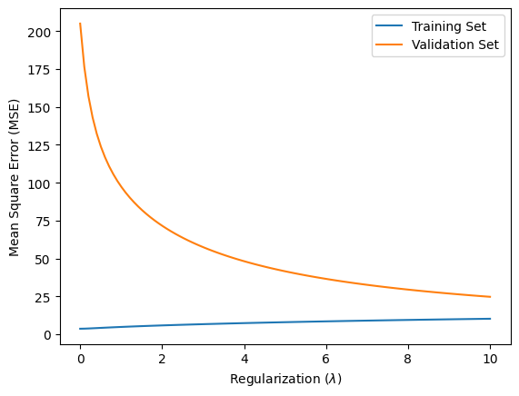
First, normalize the data and then fit a Ridge regression model to the training data using sklearn.linear_model.Ridge. Plot the training set and validation set mean square error versus the regularization parameter \(\lambda\) as \(\lambda\) is varied from \(0\) to \(10\) (Note: \(\lambda\) is the argument alpha in the Ridge object). You should see that the model overfits the training set for \(\lambda = 0\) (no regularization), but as \(\lambda\) increases the validation set error should decrease.

---

Hint: To fit a Ridge regression model to a normalized data matrix Z_train and labels y_train, and make predictions on a validation dataset Z_valdation, you can use the following code:

from sklearn.linear_model import Ridge

lambda_reg = 0.5 # regularization parameter

# fit model to training data:
model = Ridge(alpha=lambda_reg)
model.fit(Z_train,y_train)

# make predictions on validation set data:
yhat_validation = model.predict(Z_validation)

Solutions:

Exercise 1: Computing the Moore-Penrose Inverse

Show code cell content Hide code cell content

import numpy as np

# given data matrix (X) and target vector (y):
y_vector = np.array(np.arange(8)).T # shape: (8,)
X_matrix = np.hstack([
    np.ones((8,1)), 
    np.sqrt(np.arange(8*4)).reshape(8,4)
]) # shape: (8,5)

# compute weights using np.linalg.pinv:
w_numpy = np.linalg.pinv(X_matrix) @ y_vector

# print np.pinv weight vector:
print('w (computed using np.pinv):')
print(w_numpy)

# compute weight vector using the formula:
X_pinv = np.linalg.inv(X_matrix.T @ X_matrix) @ X_matrix.T
w_formula = X_pinv @ y_vector

# print formula weight vector:
print('w (computed with formula):')
print(w_formula)

# compute the MSE of the linear regression model:
yhat_vector = X_matrix @ w_numpy
mse = np.mean( (yhat_vector - y_vector)**2 )
print('\nMean Square Error: ', mse)

w (computed using np.pinv):
[ -19.13512146  -12.39983252  184.11013704 -396.71057275  228.66445803]
w (computed with formula):
[ -19.13512504  -12.39983948  184.11022702 -396.71075017  228.66455279]

Mean Square Error:  6.017971108799712e-05

Exercise 2: Regularized Linear Regression

Show code cell content Hide code cell content

import numpy as np
from sklearn.preprocessing import StandardScaler
from sklearn.linear_model import Ridge 

def generate_X(n_data):
    np.random.seed(0)
    return np.array([
        np.random.uniform(0,10,n_data)*(10**(-n/4))
        for n in range(40)
    ]).T

def generate_y(X, noise=0.5):
    np.random.seed(0)
    return np.array([
        np.sum([ 2e-6*(10**(n/4))*x_n for n,x_n in enumerate(x) ]) + \
            np.random.normal(0,noise)
        for x in X
    ])

# generate training set:
X_train = generate_X(45)
y_train = generate_y(X_train, noise=5.0)


# generate validation set:
X_validation = generate_X(20)
y_validation = generate_y(X_validation, noise=0.0)

# normalize training and validation sets:
scaler = StandardScaler()
scaler.fit(X_train)
Z_train = scaler.transform(X_train)
Z_validation = scaler.transform(X_validation)

lambda_values = np.linspace(0,10.0, 100)

train_mse_values = []
validation_mse_values = []

for lambda_reg in lambda_values:
    ridge_model = Ridge(alpha=lambda_reg)
    ridge_model.fit(Z_train, y_train)
    

    # make prediction and evaluate training set error:
    yhat_train = ridge_model.predict(Z_train)
    mse_train = np.mean((yhat_train - y_train)**2)

    # make predictions and evaluate validation set error:
    yhat_validation = ridge_model.predict(Z_validation)
    mse_validation = np.mean((yhat_validation - y_validation)**2)
    
    # record results:
    train_mse_values.append(mse_train)
    validation_mse_values.append(mse_validation)

# plot ridge regression results:
plt.figure()
plt.plot(lambda_values, train_mse_values, label='Training Set')
plt.plot(lambda_values, validation_mse_values, label='Validation Set')
plt.ylabel('Mean Square Error (MSE)')
plt.xlabel(r'Regularization ($\lambda$)')
plt.legend()
plt.show()