Training Neural Networks

Training Neural Networks#

In the previous sections, we used the Scikit-learn (sklearn) package to provide functionality for creating and fitting models to data. Although Scikit-learn does have some functionality for fitting basic neural networks to data, it does not provide an interface to larger neural network models, especially those used in deep learning. To handle these larger models, we will need to use a package that is designed specifically for neural networks or similar large models. Currently, the most popular packages are Pytorch and Tensorflow.

Since both packages serve roughly the same purpose, you only need to become familiar with one or the other. Pytorch is more commonly used in academic research, as it is easier to learn and integrates very well with the Python programming language. On the other hand, Tensorflow is more commonly used in industry due the fact that it integrates well across different platforms and programming languages. In this workshop, we will use Pytorch due to its popularity in the research community.

Review: Gradient Descent#

The most effective way of fitting neural networks to data is via the method of gradient descent, which makes iterative adjustments to the weights of the model in order to decrease the model loss function \(\mathcal{E}(f)\). As we learned in the Fitting Supervised Models section, this is done by adjusting the weights in the direction of \(-\nabla_w \mathcal{E}(f)\), which is a vector of weight adjustments that “points” in the direction of greatest decrease of \(\mathcal{E}(f)\). Specifically, for a weight configuration at timestep \(t\), the updated weight configuration in timestep \(t+1\) is computed according to

\[\mathbf{w}^{(t+1)} = \mathbf{w}^{(t)} + \eta \frac{-\nabla_w \mathcal{E}(f)}{\lVert{-\nabla_w \mathcal{E}(f)}\rVert},\]

where \(\eta\) is a constant called the learning rate. It determines the size of the weight adjustment during each timestep. Recall that if \(\eta\) is set too high, the model loss \(\mathcal{E}(f)\) may “overstep” a local minimum between timesteps; however, if \(\eta\) is set too small than the model may take a very long time to converge.

Backpropagation and Neural Networks#

Specifically, we recall that for a single data point loss function \(E(y,\hat{y})\), the gradient of the corresponding model loss function \(\mathcal{E}(f)\) on a dataset \(\{(\mathbf{x}, y)\}\) with respect to the model weights takes the form:

\[\nabla_w \mathcal{E}(f) = \frac{1}{N}\sum_{n=1}^N \frac{\partial E}{\partial \hat{y}}(f(\mathbf{x}_n), y_n) \cdot \nabla_w f(\mathbf{x}_n)\]

We can see that in order to successfully train a neural network model, the loss function \(E\) must be differentiable and the entire neural network \(f\) must be completely differentiable with respect to the weights. Furthermore, while the term \(\frac{\partial E}{\partial \hat{y}}(f(\mathbf{x}_n), y_n)\) may be easy to compute for each datapoint, computing \(\nabla_w f(\mathbf{x})\) may require a substantial amount of calculus and linear algebra to compute.

Fortunately, machine learning frameworks like Pytorch and Tensorflow can compute the gradients of differentiable functions automatically, provided that they are built using functions with known derivatives and Python arithmetic operations (such as +, -, *, /, etc.). The process by which \(\nabla_w\) is computed for the weights in each layer in the neural network is called backpropagation, because it computes the gradient of the weights starting with the last layer and working backwards through the layers of the network in an efficient manner.

Batch Gradient Descent#

Sometimes, our dataset may be too large to compute \(\nabla_w \mathcal{E}(f)\) across all \((\mathbf{x}_n, y_n)\) pairs for each time step of gradient descent. One solution to this is to randomly split the dataset into “chunks” of a fixed size and perform gradient-based weight updates on each chunk of the dataset. These fixed-size chunks of data are usually referred to as batches, and their size is called the batch size.

The number of steps that have elapsed while fitting a neural to network to a large dataset is often measured in epochs. During each epoch, the model iterates over each batch in the dataset, evaluates the loss on the batch, and updates the model weights. In other words, the number of epochs that have passed while training the model indicates how many times the model has “seen” each example in the dataset. This process of performing gradient descent on batches of data is called batch gradient descent. Below, we give a brief summary of this is typically done:

Randomly shuffle the data and partition it into batches of a fixed size.

For each epoch, do the following:

(Optional): Shuffle the batches in a random order.

For each batch in the dataset, apply a weight update.

Repeat Steps 2-4 until either the training error converges or the validation error is minimized.

Basic Feed-Forward Network with Pytorch#

In the previous section, we learned about a standard feed-forward neural network, which consists of two layers of neurons: a hidden layer containing many neurons followed by an output layer containing the same number of neurons as the output vector \(\mathbf{y}\) to be predicted. To give a basic example of how this neural network can be implemented in Pytorch, let’s fit a neural neural network \(f(\mathbf{x}): \mathbb{R}^2 \rightarrow \mathbb{R}\) to the following function:

\[y = g(\mathbf{x}) = \frac{\sin\left(\sqrt{x_1^2 + x_2^2}\right)}{\sqrt{x_1^2 + x_2^2}}\]

(We plotted this function earlier in the Data Visualization with Matplotlib section.)

To begin, let’s import Pytorch and write a FeedForwardNN class that represents a standard feed-forward neural network. This class will inherit from torch.nn.Module, a class which represents a Pytorch-compatible model. Since the function \(g(\mathbf{x})\) above has \(y\) bounded from \(-1\) to \(+1\) we will use the hyperbolic tangent activation function (\(\sigma(x) = \tanh(x)\)) for the hidden and output layers:

import torch
import torch.nn as nn

# Define the neural network class
class FeedForwardNN(nn.Module):
    """
    torch.nn Module for a standard feed-forward
    neural network with a single hidden layer
    """

    def __init__(self, input_size, hidden_size, output_size):
        """ Constructs a simple feed-forward neural network """
        super(FeedForwardNN, self).__init__()

        # Define layer 1 weights (input -> hidden layer):
        self.hidden_layer = nn.Linear(input_size, hidden_size)

        # define hidden layer activation function:
        self.hidden_activation = nn.Tanh()

        # define layer 2 weights (hidden layer -> output layer):
        self.output_layer = nn.Linear(hidden_size, output_size)

        # define output activation:
        self.output_activation = nn.Tanh()
    
    def forward(self, x):
        """ computes the neural network prediction """
        x2 = self.hidden_layer(x)
        x3 = self.hidden_activation(x2)
        x4 = self.output_layer(x3)
        out = self.output_activation(x4)
        
        return out

Next, we will generate a dataset of points sampled from \(g(x)\). In this example, we will not be concerned with splitting the data into train, validation, and test sets, but we will normalize the data.

data_z shape: (2500, 2)
data_y shape: (2500, 1)

In Pytorch, muti-dimensional data must be stored using the torch.tensor data type. Pytorch tensors are essentially equivalent to numpy arrays, but they must be converted prior to using them as input to the model. To help us manage creating a dataset from a Numpy array, we will write a class called NumpyDataset that inherits from the torch.utils.data.Dataset class. This will allow us a convenient way to iterate over the data when we are fitting our model:

from torch.utils.data import Dataset

# Define a custom dataset class
class NumpyDataset(Dataset):
    def __init__(self, data_x, data_y):
        self.data_x = torch.tensor(data_x, dtype=torch.float32)
        self.data_y = torch.tensor(data_y, dtype=torch.float32)
        
    def __len__(self):
        return len(self.data_x)
    
    def __getitem__(self, idx):
        x = self.data_x[idx]
        y = self.data_y[idx]
        return x, y

Next, we will configure some neural network parameters, such as the input size (must be 2), the number of hidden neurons, and the number of output neurons (must be 1). We will also configure training parameters, such as the learning rate, the batch size, and how many epochs we think we need to fit the model:

# neural network parameters:
input_size = 2
hidden_size = 80
output_size = 1

# training parameters:
learning_rate = 1e-2
batch_size = 200
n_epochs = 400

Using the FeedForwardNN class and NumpyDataset classes we created, we will create an instance of our model using the parameters set above. In order to partition the data into batches, we will use the torch.utils.data.DataLoader class:

from torch.utils.data import DataLoader
import torch.nn as nn
import torch.optim as optim

# create the model:
model = FeedForwardNN(input_size, hidden_size, output_size)

# construct dataset and data loader:
dataset = NumpyDataset(data_z, data_y)
data_loader = DataLoader(dataset, batch_size=batch_size, shuffle=True)

Next, we will set the loss function as the mean square error loss, and add a gradient descent optimizer called Adam (Adaptive moment estimation).

# specify loss function and optimizer:
loss_function = nn.MSELoss()
optimizer = optim.Adam(model.parameters(), lr=learning_rate)

Using the following code, we will define the training loop of our model, where during each epoch we iterate over eatch batch in the dataset and update the model weights. In order to keep track of the average model loss for each epoch, we will use a list called loss_history:

# list to record loss over time:
loss_history = []

for epoch in range(n_epochs):
    
    # apply stochastic gradient descent step to each batch in dataset:
    epoch_losses = []
    for z_batch, y_batch in data_loader:
        
        # zero optimizer gradient:
        optimizer.zero_grad()

        # generate batch prediction
        y_hat_batch = model(z_batch)
        
        # compute loss:
        loss = loss_function(y_hat_batch, y_batch)
        epoch_losses.append(loss.item())

        # backpropagate loss:
        loss.backward()
        optimizer.step()
    
    loss_history.append(np.mean(epoch_losses))

After training the model, we can visualize the loss as follows:

import matplotlib.pyplot as plt

plt.figure()
plt.grid()
plt.plot(loss_history)
plt.xlabel('Epoch')
plt.ylabel('Model Loss (Mean Square Error)')
plt.show()

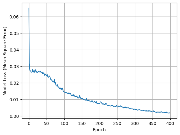
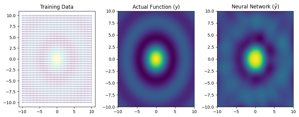
../_images/e2b3d80628580a86a1a0dd43b9fc7fb48f8cb15668949c56131ef3514f5e9dc1.png

From inspecting the plot, we can see that the mean square error has converged to a value close to \(0\). Using the following code, we can visualize how well the prediction surface of the neural network (\(\hat{y}\)) compares with the actual function is was fit to: